

438
A. V. Dvornichenko and O. M. Shchokotova
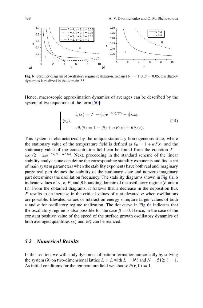
Fig. 6 Stability diagram of oscillatory regime realization. In panel b ν = 1.0, β = 0.05. Oscillatory
dynamics is realized in the domain I I
Hence, macroscopic approximation dynamics of averages can be described by the
system of two equations of the form [50]:
⎧
⎪ ⎨
⎪ ⎩
∂ t = F − −x
−ε
−
1
2
λx 0 ,
φ
ν∂ t = 1 − −θ + α F + β∂ t
(14)
This system is characterized by the unique stationary homogeneous state, where
the stationary value of the temperature field is defined as θ 0 = 1 + α F x 0 and the
stationary value of the concentration field can be found from the equation F −
λx 0 /2 = x 0 e
−εx 0 /(1+α F x 0 ) . Next, proceeding in the standard scheme of the linear
stability analysis one can define the corresponding stability exponents and find a set
of main system parameters when the stability exponents have both real and imaginary
parts: real part defines the stability of the stationary state and nonzero imaginary
part determines the oscillation frequency. The stability diagrams shown in Fig. 6a, b
indicate values of α, ν, F, and β bounding domain of the oscillatory regime (domain
II). From the obtained diagrams, it follows that a decrease in the deposition flux
F results to an increase in the critical values of ν at elevated α when oscillations
are possible. Elevated values of interaction energy ε require larger values of both
ν and α for oscillatory regime realization. The dot curve in Fig. 6a indicates that
the oscillatory regime is also possible for the case β = 0. Hence, in the case of the
constant positive value of the speed of the surface growth oscillatory dynamics of
both averaged quantities and can be realized.
5.2 Numerical Results
In this section, we will study dynamics of pattern formation numerically by solving
the system (9) on two-dimensional lattice L × L with L = N and N = 512; = 1.
As initial conditions for the temperature field we choose θ(r, 0) = 1.
A. V. Dvornichenko and O. M. Shchokotova
Fig. 6 Stability diagram of oscillatory regime realization. In panel b ν = 1.0, β = 0.05. Oscillatory
dynamics is realized in the domain I I
Hence, macroscopic approximation dynamics of averages can be described by the
system of two equations of the form [50]:
⎧
⎪ ⎨
⎪ ⎩
∂ t = F − −x
−ε
−
1
2
λx 0 ,
φ
ν∂ t = 1 − −θ + α F + β∂ t
(14)
This system is characterized by the unique stationary homogeneous state, where
the stationary value of the temperature field is defined as θ 0 = 1 + α F x 0 and the
stationary value of the concentration field can be found from the equation F −
λx 0 /2 = x 0 e
−εx 0 /(1+α F x 0 ) . Next, proceeding in the standard scheme of the linear
stability analysis one can define the corresponding stability exponents and find a set
of main system parameters when the stability exponents have both real and imaginary
parts: real part defines the stability of the stationary state and nonzero imaginary
part determines the oscillation frequency. The stability diagrams shown in Fig. 6a, b
indicate values of α, ν, F, and β bounding domain of the oscillatory regime (domain
II). From the obtained diagrams, it follows that a decrease in the deposition flux
F results to an increase in the critical values of ν at elevated α when oscillations
are possible. Elevated values of interaction energy ε require larger values of both
ν and α for oscillatory regime realization. The dot curve in Fig. 6a indicates that
the oscillatory regime is also possible for the case β = 0. Hence, in the case of the
constant positive value of the speed of the surface growth oscillatory dynamics of
both averaged quantities and can be realized.
5.2 Numerical Results
In this section, we will study dynamics of pattern formation numerically by solving
the system (9) on two-dimensional lattice L × L with L = N and N = 512; = 1.
As initial conditions for the temperature field we choose θ(r, 0) = 1.