

Theoretical Modeling of Laser-Stimulated Nanostructures
281
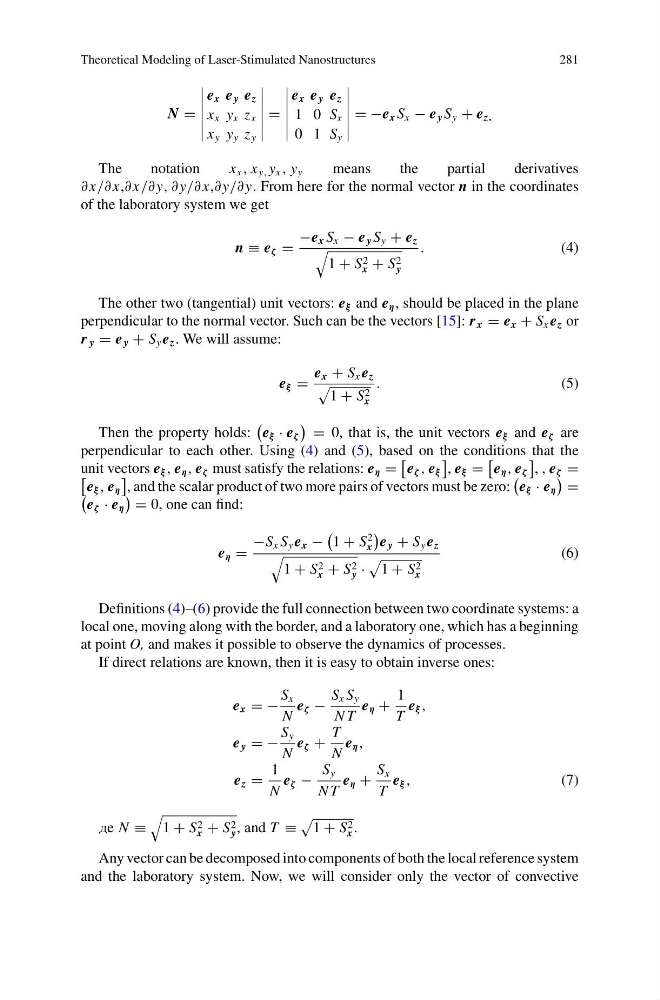
N =
e x e y e z
x x y x z x
x y y y z y
=
e x e y e z
1 0 S x
0 1 S y
= −e x S x − e y S y + e z.
The
notation
x x , x y, y x , y y
means
the
partial
derivatives
∂ x/∂ x,∂ x/∂ y, ∂y/∂ x,∂ y/∂ y. From here for the normal vector n in the coordinates
of the laboratory system we get
n ≡ e ζ =
−e x S x − e y S y + e z
1 + S 2
x + S 2
y
.
(4)
The other two (tangential) unit vectors: e ξ and e η , should be placed in the plane
perpendicular to the normal vector. Such can be the vectors [15]: r x = e x + S x e z or
r y = e y + S y e z . We will assume:
e ξ =
e x + S x e z
1 + S 2
x
.
(5)
Then the property holds:
e ξ · e ζ
= 0, that is, the unit vectors e ξ and e ζ are
perpendicular to each other. Using (4) and (5), based on the conditions that the
unit vectors e ξ , e η , e ζ must satisfy the relations: e η =
e ζ , e ξ
, e ξ =
e η , e ζ
, , e ζ =
e ξ , e η
, and the scalar product of two more pairs of vectors must be zero:
e ξ · e η
=
e ζ · e η
= 0, one can find:
e η =
−S x S y e x −
1 + S
2
x
e y + S y e z
1 + S 2
x + S 2
y ·
1 + S 2
x
(6)
Definitions (4)–(6) provide the full connection between two coordinate systems: a
local one, moving along with the border, and a laboratory one, which has a beginning
at point O, and makes it possible to observe the dynamics of processes.
If direct relations are known, then it is easy to obtain inverse ones:
e x = −
S x
N
e ζ −
S x S y
N T
e η +
1
T
e ξ ,
e y = −
S y
N
e ζ +
T
N
e η ,
e z =
1
N
e ζ −
S y
N T
e η +
S x
T
e ξ ,
(7)
de N ≡
1 + S 2
x + S 2
y , and T ≡
1 + S 2
x .
Any vector can be decomposed into components of both the local reference system
and the laboratory system. Now, we will consider only the vector of convective
281
N =
e x e y e z
x x y x z x
x y y y z y
=
e x e y e z
1 0 S x
0 1 S y
= −e x S x − e y S y + e z.
The
notation
x x , x y, y x , y y
means
the
partial
derivatives
∂ x/∂ x,∂ x/∂ y, ∂y/∂ x,∂ y/∂ y. From here for the normal vector n in the coordinates
of the laboratory system we get
n ≡ e ζ =
−e x S x − e y S y + e z
1 + S 2
x + S 2
y
.
(4)
The other two (tangential) unit vectors: e ξ and e η , should be placed in the plane
perpendicular to the normal vector. Such can be the vectors [15]: r x = e x + S x e z or
r y = e y + S y e z . We will assume:
e ξ =
e x + S x e z
1 + S 2
x
.
(5)
Then the property holds:
e ξ · e ζ
= 0, that is, the unit vectors e ξ and e ζ are
perpendicular to each other. Using (4) and (5), based on the conditions that the
unit vectors e ξ , e η , e ζ must satisfy the relations: e η =
e ζ , e ξ
, e ξ =
e η , e ζ
, , e ζ =
e ξ , e η
, and the scalar product of two more pairs of vectors must be zero:
e ξ · e η
=
e ζ · e η
= 0, one can find:
e η =
−S x S y e x −
1 + S
2
x
e y + S y e z
1 + S 2
x + S 2
y ·
1 + S 2
x
(6)
Definitions (4)–(6) provide the full connection between two coordinate systems: a
local one, moving along with the border, and a laboratory one, which has a beginning
at point O, and makes it possible to observe the dynamics of processes.
If direct relations are known, then it is easy to obtain inverse ones:
e x = −
S x
N
e ζ −
S x S y
N T
e η +
1
T
e ξ ,
e y = −
S y
N
e ζ +
T
N
e η ,
e z =
1
N
e ζ −
S y
N T
e η +
S x
T
e ξ ,
(7)
de N ≡
1 + S 2
x + S 2
y , and T ≡
1 + S 2
x .
Any vector can be decomposed into components of both the local reference system
and the laboratory system. Now, we will consider only the vector of convective