

90
4 Multi-Degree of Freedom (MDOF) Systems
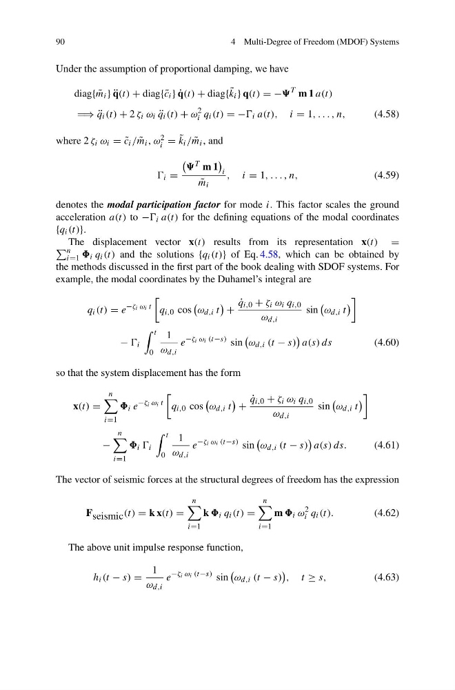
Under the assumption of proportional damping, we have
diag{ ˜
m i } ¨
q(t) + diag{ ˜
c i } ˙
q(t) + diag{ ˜
k i } q(t) = −
T m 1 a(t)
⇒ ¨
q i (t) + 2 ζ i ω i ¨
q i (t) + ω
2
i q i (t) = − i a(t), i = 1, . . . , n,
(4.58)
where 2 ζ i ω i = ˜
c i / ˜
m i , ω 2
i = ˜
k i / ˜
m i , and
i =
T m 1
i
˜
m i
, i = 1, . . . , n,
(4.59)
denotes the modal participation factor for mode i. This factor scales the ground
acceleration a(t) to − i a(t) for the defining equations of the modal coordinates
{q i (t)}.
The displacement vector x(t) results from its representation x(t) =
n
i=1 i q i (t) and the solutions {q i (t)} of Eq. 4.58, which can be obtained by
the methods discussed in the first part of the book dealing with SDOF systems. For
example, the modal coordinates by the Duhamel’s integral are
q i (t) = e
−ζ i ω i t
q i,0 cos
ω d,i t
+
˙
q i,0 + ζ i ω i q i,0
ω d,i
sin
ω d,i t
− i
t
0
1
ω d,i
e
−ζ i ω i (t−s) sin
ω d,i (t − s)
a(s) ds
(4.60)
so that the system displacement has the form
x(t) =
n
i=1
i e
−ζ i ω i t
q i,0 cos
ω d,i t
+
˙
q i,0 + ζ i ω i q i,0
ω d,i
sin
ω d,i t
−
n
i=1
i i
t
0
1
ω d,i
e
−ζ i ω i (t−s) sin
ω d,i (t − s)
a(s) ds.
(4.61)
The vector of seismic forces at the structural degrees of freedom has the expression
F seismic (t) = k x(t) =
n
i=1
k i q i (t) =
n
i=1
m i ω
2
i q i (t).
(4.62)
The above unit impulse response function,
h i (t − s) =
1
ω d,i
e
−ζ i ω i (t−s) sin
ω d,i (t − s)
, t ≥ s,
(4.63)
4 Multi-Degree of Freedom (MDOF) Systems
Under the assumption of proportional damping, we have
diag{ ˜
m i } ¨
q(t) + diag{ ˜
c i } ˙
q(t) + diag{ ˜
k i } q(t) = −
T m 1 a(t)
⇒ ¨
q i (t) + 2 ζ i ω i ¨
q i (t) + ω
2
i q i (t) = − i a(t), i = 1, . . . , n,
(4.58)
where 2 ζ i ω i = ˜
c i / ˜
m i , ω 2
i = ˜
k i / ˜
m i , and
i =
T m 1
i
˜
m i
, i = 1, . . . , n,
(4.59)
denotes the modal participation factor for mode i. This factor scales the ground
acceleration a(t) to − i a(t) for the defining equations of the modal coordinates
{q i (t)}.
The displacement vector x(t) results from its representation x(t) =
n
i=1 i q i (t) and the solutions {q i (t)} of Eq. 4.58, which can be obtained by
the methods discussed in the first part of the book dealing with SDOF systems. For
example, the modal coordinates by the Duhamel’s integral are
q i (t) = e
−ζ i ω i t
q i,0 cos
ω d,i t
+
˙
q i,0 + ζ i ω i q i,0
ω d,i
sin
ω d,i t
− i
t
0
1
ω d,i
e
−ζ i ω i (t−s) sin
ω d,i (t − s)
a(s) ds
(4.60)
so that the system displacement has the form
x(t) =
n
i=1
i e
−ζ i ω i t
q i,0 cos
ω d,i t
+
˙
q i,0 + ζ i ω i q i,0
ω d,i
sin
ω d,i t
−
n
i=1
i i
t
0
1
ω d,i
e
−ζ i ω i (t−s) sin
ω d,i (t − s)
a(s) ds.
(4.61)
The vector of seismic forces at the structural degrees of freedom has the expression
F seismic (t) = k x(t) =
n
i=1
k i q i (t) =
n
i=1
m i ω
2
i q i (t).
(4.62)
The above unit impulse response function,
h i (t − s) =
1
ω d,i
e
−ζ i ω i (t−s) sin
ω d,i (t − s)
, t ≥ s,
(4.63)