

4.4 Time Domain Analysis: Proportional Damping
83
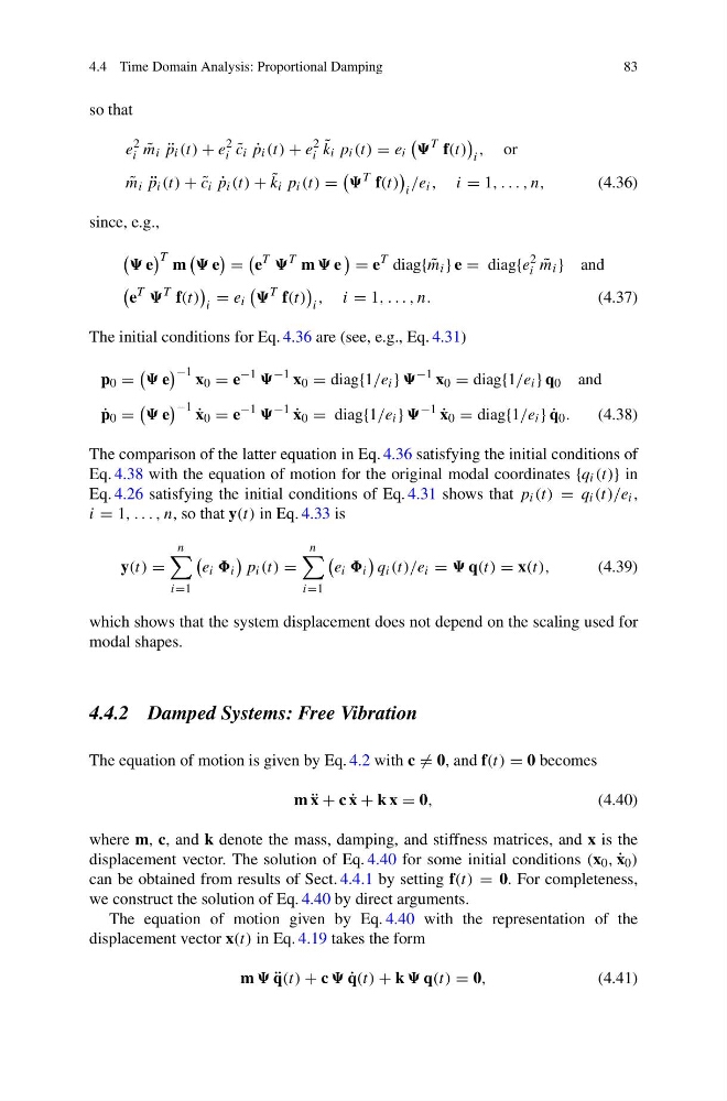
so that
e
2
i ˜
m i ¨
p i (t) + e
2
i ˜
c i ˙
p i (t) + e
2
i
˜
k i p i (t) = e i
T f(t)
i
, or
˜
m i ¨
p i (t) + ˜
c i ˙
p i (t) + ˜
k i p i (t) =
T f(t)
i
/e i , i = 1, . . . , n,
(4.36)
since, e.g.,
e
T m
e
=
e
T
T m e
= e
T diag{ ˜
m i } e = diag{e
2
i ˜
m i } and
e
T
T f(t)
i
= e i
T f(t)
i
, i = 1, . . . , n.
(4.37)
The initial conditions for Eq. 4.36 are (see, e.g., Eq. 4.31)
p 0 =
e
−1 x 0 = e
−1
−1 x 0 = diag{1/e i }
−1 x 0 = diag{1/e i } q 0 and
˙
p 0 =
e
−1 ˙
x 0 = e
−1
−1
˙
x 0 = diag{1/e i }
−1
˙
x 0 = diag{1/e i } ˙
q 0 .
(4.38)
The comparison of the latter equation in Eq. 4.36 satisfying the initial conditions of
Eq. 4.38 with the equation of motion for the original modal coordinates {q i (t)} in
Eq. 4.26 satisfying the initial conditions of Eq. 4.31 shows that p i (t) = q i (t)/e i ,
i = 1, . . . , n, so that y(t) in Eq. 4.33 is
y(t) =
n
i=1
e i i
p i (t) =
n
i=1
e i i
q i (t)/e i = q(t) = x(t),
(4.39)
which shows that the system displacement does not depend on the scaling used for
modal shapes.
4.4.2 Damped Systems: Free Vibration
The equation of motion is given by Eq. 4.2 with c = 0, and f(t) = 0 becomes
m ¨
x + c ˙
x + k x = 0,
(4.40)
where m, c, and k denote the mass, damping, and stiffness matrices, and x is the
displacement vector. The solution of Eq. 4.40 for some initial conditions (x 0 , ˙
x 0 )
can be obtained from results of Sect. 4.4.1 by setting f(t) = 0. For completeness,
we construct the solution of Eq. 4.40 by direct arguments.
The equation of motion given by Eq. 4.40 with the representation of the
displacement vector x(t) in Eq. 4.19 takes the form
m ¨
q(t) + c ˙
q(t) + k q(t) = 0,
(4.41)
83
so that
e
2
i ˜
m i ¨
p i (t) + e
2
i ˜
c i ˙
p i (t) + e
2
i
˜
k i p i (t) = e i
T f(t)
i
, or
˜
m i ¨
p i (t) + ˜
c i ˙
p i (t) + ˜
k i p i (t) =
T f(t)
i
/e i , i = 1, . . . , n,
(4.36)
since, e.g.,
e
T m
e
=
e
T
T m e
= e
T diag{ ˜
m i } e = diag{e
2
i ˜
m i } and
e
T
T f(t)
i
= e i
T f(t)
i
, i = 1, . . . , n.
(4.37)
The initial conditions for Eq. 4.36 are (see, e.g., Eq. 4.31)
p 0 =
e
−1 x 0 = e
−1
−1 x 0 = diag{1/e i }
−1 x 0 = diag{1/e i } q 0 and
˙
p 0 =
e
−1 ˙
x 0 = e
−1
−1
˙
x 0 = diag{1/e i }
−1
˙
x 0 = diag{1/e i } ˙
q 0 .
(4.38)
The comparison of the latter equation in Eq. 4.36 satisfying the initial conditions of
Eq. 4.38 with the equation of motion for the original modal coordinates {q i (t)} in
Eq. 4.26 satisfying the initial conditions of Eq. 4.31 shows that p i (t) = q i (t)/e i ,
i = 1, . . . , n, so that y(t) in Eq. 4.33 is
y(t) =
n
i=1
e i i
p i (t) =
n
i=1
e i i
q i (t)/e i = q(t) = x(t),
(4.39)
which shows that the system displacement does not depend on the scaling used for
modal shapes.
4.4.2 Damped Systems: Free Vibration
The equation of motion is given by Eq. 4.2 with c = 0, and f(t) = 0 becomes
m ¨
x + c ˙
x + k x = 0,
(4.40)
where m, c, and k denote the mass, damping, and stiffness matrices, and x is the
displacement vector. The solution of Eq. 4.40 for some initial conditions (x 0 , ˙
x 0 )
can be obtained from results of Sect. 4.4.1 by setting f(t) = 0. For completeness,
we construct the solution of Eq. 4.40 by direct arguments.
The equation of motion given by Eq. 4.40 with the representation of the
displacement vector x(t) in Eq. 4.19 takes the form
m ¨
q(t) + c ˙
q(t) + k q(t) = 0,
(4.41)