

4.3 Classical Modal Analysis
71
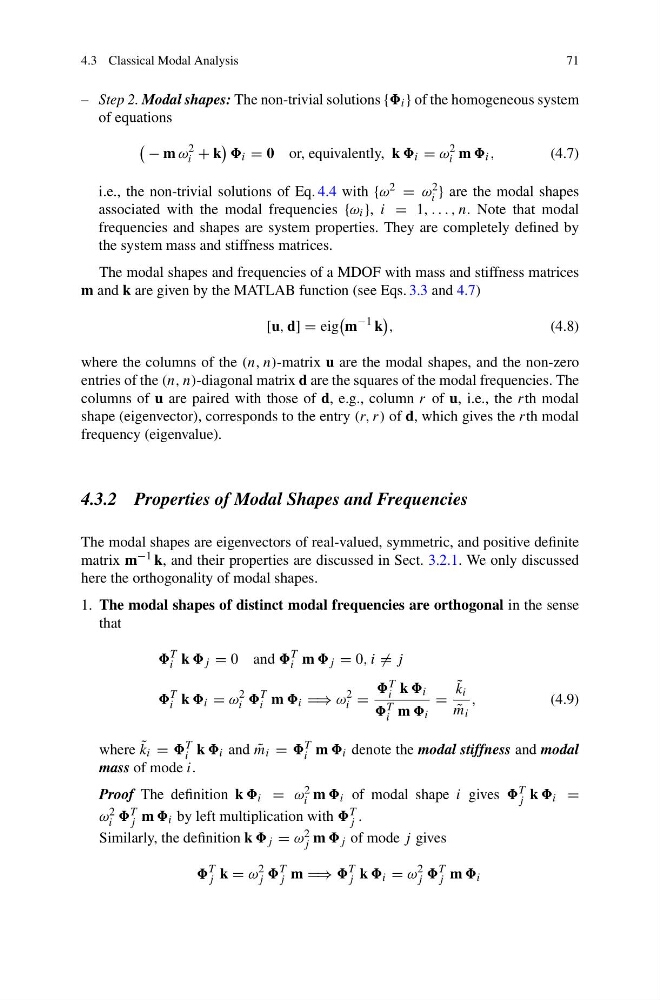
– Step 2. Modal shapes: The non-trivial solutions { i } of the homogeneous system
of equations
− m ω
2
i + k
i = 0 or, equivalently, k i = ω
2
i m i ,
(4.7)
i.e., the non-trivial solutions of Eq. 4.4 with {ω 2 = ω 2
i } are the modal shapes
associated with the modal frequencies {ω i }, i = 1, . . . , n. Note that modal
frequencies and shapes are system properties. They are completely defined by
the system mass and stiffness matrices.
The modal shapes and frequencies of a MDOF with mass and stiffness matrices
m and k are given by the MATLAB function (see Eqs. 3.3 and 4.7)
[u, d] = eig
m
−1 k
,
(4.8)
where the columns of the (n, n)-matrix u are the modal shapes, and the non-zero
entries of the (n, n)-diagonal matrix d are the squares of the modal frequencies. The
columns of u are paired with those of d, e.g., column r of u, i.e., the rth modal
shape (eigenvector), corresponds to the entry (r, r) of d, which gives the rth modal
frequency (eigenvalue).
4.3.2 Properties of Modal Shapes and Frequencies
The modal shapes are eigenvectors of real-valued, symmetric, and positive definite
matrix m −1 k, and their properties are discussed in Sect. 3.2.1. We only discussed
here the orthogonality of modal shapes.
1. The modal shapes of distinct modal frequencies are orthogonal in the sense
that
T
i k j = 0 and
T
i m j = 0, i = j
T
i k i = ω
2
i
T
i m i ⇒ ω
2
i =
T
i k i
T
i m i
=
˜
k i
˜
m i
,
(4.9)
where ˜
k i = T
i k i and ˜
m i = T
i m i denote the modal stiffness and modal
mass of mode i.
Proof The definition k i = ω 2
i m i of modal shape i gives T
j k i =
ω 2
i T
j m i by left multiplication with T
j .
Similarly, the definition k j = ω 2
j m j of mode j gives
T
j k = ω
2
j
T
j m ⇒
T
j k i = ω
2
j
T
j m i
71
– Step 2. Modal shapes: The non-trivial solutions { i } of the homogeneous system
of equations
− m ω
2
i + k
i = 0 or, equivalently, k i = ω
2
i m i ,
(4.7)
i.e., the non-trivial solutions of Eq. 4.4 with {ω 2 = ω 2
i } are the modal shapes
associated with the modal frequencies {ω i }, i = 1, . . . , n. Note that modal
frequencies and shapes are system properties. They are completely defined by
the system mass and stiffness matrices.
The modal shapes and frequencies of a MDOF with mass and stiffness matrices
m and k are given by the MATLAB function (see Eqs. 3.3 and 4.7)
[u, d] = eig
m
−1 k
,
(4.8)
where the columns of the (n, n)-matrix u are the modal shapes, and the non-zero
entries of the (n, n)-diagonal matrix d are the squares of the modal frequencies. The
columns of u are paired with those of d, e.g., column r of u, i.e., the rth modal
shape (eigenvector), corresponds to the entry (r, r) of d, which gives the rth modal
frequency (eigenvalue).
4.3.2 Properties of Modal Shapes and Frequencies
The modal shapes are eigenvectors of real-valued, symmetric, and positive definite
matrix m −1 k, and their properties are discussed in Sect. 3.2.1. We only discussed
here the orthogonality of modal shapes.
1. The modal shapes of distinct modal frequencies are orthogonal in the sense
that
T
i k j = 0 and
T
i m j = 0, i = j
T
i k i = ω
2
i
T
i m i ⇒ ω
2
i =
T
i k i
T
i m i
=
˜
k i
˜
m i
,
(4.9)
where ˜
k i = T
i k i and ˜
m i = T
i m i denote the modal stiffness and modal
mass of mode i.
Proof The definition k i = ω 2
i m i of modal shape i gives T
j k i =
ω 2
i T
j m i by left multiplication with T
j .
Similarly, the definition k j = ω 2
j m j of mode j gives
T
j k = ω
2
j
T
j m ⇒
T
j k i = ω
2
j
T
j m i