

42
2 Single Degree of Freedom (SDOF) Systems
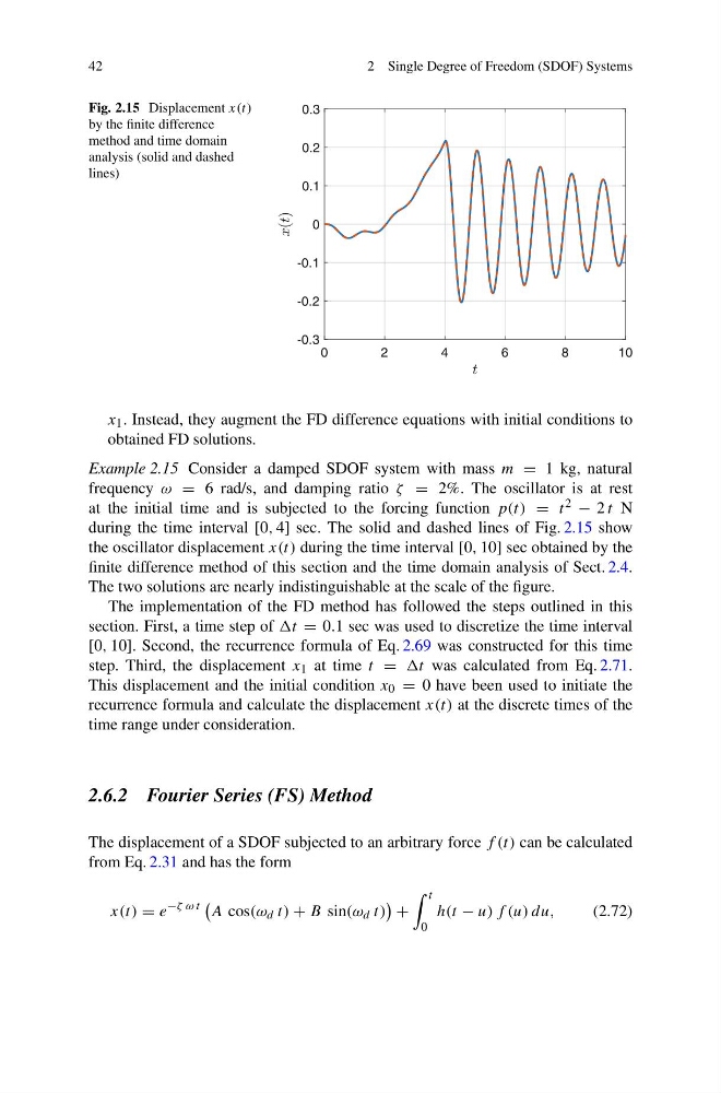
Fig. 2.15 Displacement x(t)
by the finite difference
method and time domain
analysis (solid and dashed
lines)
0
2
4
6
8
1 0
-0.3
-0.2
-0.1
0
0.1
0.2
0.3
x 1 . Instead, they augment the FD difference equations with initial conditions to
obtained FD solutions.
Example 2.15 Consider a damped SDOF system with mass m = 1 kg, natural
frequency ω = 6 rad/s, and damping ratio ζ = 2%. The oscillator is at rest
at the initial time and is subjected to the forcing function p(t) = t 2 − 2 t N
during the time interval [0, 4] sec. The solid and dashed lines of Fig. 2.15 show
the oscillator displacement x(t) during the time interval [0, 10] sec obtained by the
finite difference method of this section and the time domain analysis of Sect. 2.4.
The two solutions are nearly indistinguishable at the scale of the figure.
The implementation of the FD method has followed the steps outlined in this
section. First, a time step of t = 0.1 sec was used to discretize the time interval
[0, 10]. Second, the recurrence formula of Eq. 2.69 was constructed for this time
step. Third, the displacement x 1 at time t = t was calculated from Eq. 2.71.
This displacement and the initial condition x 0 = 0 have been used to initiate the
recurrence formula and calculate the displacement x(t) at the discrete times of the
time range under consideration.
2.6.2 Fourier Series (FS) Method
The displacement of a SDOF subjected to an arbitrary force f (t) can be calculated
from Eq. 2.31 and has the form
x(t) = e
−ζ ω t
A cos(ω d t) + B sin(ω d t)
+
t
0
h(t − u) f (u) du,
(2.72)
2 Single Degree of Freedom (SDOF) Systems
Fig. 2.15 Displacement x(t)
by the finite difference
method and time domain
analysis (solid and dashed
lines)
0
2
4
6
8
1 0
-0.3
-0.2
-0.1
0
0.1
0.2
0.3
x 1 . Instead, they augment the FD difference equations with initial conditions to
obtained FD solutions.
Example 2.15 Consider a damped SDOF system with mass m = 1 kg, natural
frequency ω = 6 rad/s, and damping ratio ζ = 2%. The oscillator is at rest
at the initial time and is subjected to the forcing function p(t) = t 2 − 2 t N
during the time interval [0, 4] sec. The solid and dashed lines of Fig. 2.15 show
the oscillator displacement x(t) during the time interval [0, 10] sec obtained by the
finite difference method of this section and the time domain analysis of Sect. 2.4.
The two solutions are nearly indistinguishable at the scale of the figure.
The implementation of the FD method has followed the steps outlined in this
section. First, a time step of t = 0.1 sec was used to discretize the time interval
[0, 10]. Second, the recurrence formula of Eq. 2.69 was constructed for this time
step. Third, the displacement x 1 at time t = t was calculated from Eq. 2.71.
This displacement and the initial condition x 0 = 0 have been used to initiate the
recurrence formula and calculate the displacement x(t) at the discrete times of the
time range under consideration.
2.6.2 Fourier Series (FS) Method
The displacement of a SDOF subjected to an arbitrary force f (t) can be calculated
from Eq. 2.31 and has the form
x(t) = e
−ζ ω t
A cos(ω d t) + B sin(ω d t)
+
t
0
h(t − u) f (u) du,
(2.72)