

2.6 Numerical Methods
41
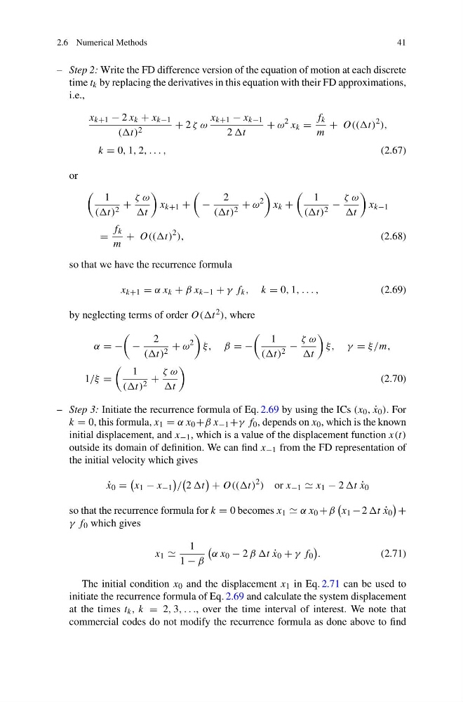
– Step 2: Write the FD difference version of the equation of motion at each discrete
time t k by replacing the derivatives in this equation with their FD approximations,
i.e.,
x k+1 − 2 x k + x k−1
((t) 2
+ 2 ζ ω
x k+1 − x k−1
2 t
+ ω
2 x k =
f k
m
+ O(((t)
2 ),
k = 0, 1, 2, . . . ,
(2.67)
or
1
((t) 2 +
ζ ω
t
x k+1 +
−
2
((t) 2 + ω
2
x k +
1
((t) 2 −
ζ ω
t
x k−1
=
f k
m
+ O(((t)
2 ),
(2.68)
so that we have the recurrence formula
x k+1 = α x k + β x k−1 + γ f k , k = 0, 1, . . . ,
(2.69)
by neglecting terms of order O((t 2 ), where
α = −
−
2
((t) 2 + ω
2
ξ, β = −
1
((t) 2 −
ζ ω
t
ξ, γ = ξ/m,
1/ξ =
1
((t) 2 +
ζ ω
t
(2.70)
– Step 3: Initiate the recurrence formula of Eq. 2.69 by using the ICs (x 0 , ˙
x 0 ). For
k = 0, this formula, x 1 = α x 0 +β x −1 +γ f 0 , depends on x 0 , which is the known
initial displacement, and x −1 , which is a value of the displacement function x(t)
outside its domain of definition. We can find x −1 from the FD representation of
the initial velocity which gives
˙
x 0 =
x 1 − x −1
/
2 t
+ O(((t)
2 ) or x −1 x 1 − 2 t ˙
x 0
so that the recurrence formula for k = 0 becomes x 1 α x 0 + β
x 1 − 2 t ˙
x 0
+
γ f 0 which gives
x 1
1
1 − β
α x 0 − 2 β βt ˙
x 0 + γ f 0
.
(2.71)
The initial condition x 0 and the displacement x 1 in Eq. 2.71 can be used to
initiate the recurrence formula of Eq. 2.69 and calculate the system displacement
at the times t k , k = 2, 3, . . ., over the time interval of interest. We note that
commercial codes do not modify the recurrence formula as done above to find
41
– Step 2: Write the FD difference version of the equation of motion at each discrete
time t k by replacing the derivatives in this equation with their FD approximations,
i.e.,
x k+1 − 2 x k + x k−1
((t) 2
+ 2 ζ ω
x k+1 − x k−1
2 t
+ ω
2 x k =
f k
m
+ O(((t)
2 ),
k = 0, 1, 2, . . . ,
(2.67)
or
1
((t) 2 +
ζ ω
t
x k+1 +
−
2
((t) 2 + ω
2
x k +
1
((t) 2 −
ζ ω
t
x k−1
=
f k
m
+ O(((t)
2 ),
(2.68)
so that we have the recurrence formula
x k+1 = α x k + β x k−1 + γ f k , k = 0, 1, . . . ,
(2.69)
by neglecting terms of order O((t 2 ), where
α = −
−
2
((t) 2 + ω
2
ξ, β = −
1
((t) 2 −
ζ ω
t
ξ, γ = ξ/m,
1/ξ =
1
((t) 2 +
ζ ω
t
(2.70)
– Step 3: Initiate the recurrence formula of Eq. 2.69 by using the ICs (x 0 , ˙
x 0 ). For
k = 0, this formula, x 1 = α x 0 +β x −1 +γ f 0 , depends on x 0 , which is the known
initial displacement, and x −1 , which is a value of the displacement function x(t)
outside its domain of definition. We can find x −1 from the FD representation of
the initial velocity which gives
˙
x 0 =
x 1 − x −1
/
2 t
+ O(((t)
2 ) or x −1 x 1 − 2 t ˙
x 0
so that the recurrence formula for k = 0 becomes x 1 α x 0 + β
x 1 − 2 t ˙
x 0
+
γ f 0 which gives
x 1
1
1 − β
α x 0 − 2 β βt ˙
x 0 + γ f 0
.
(2.71)
The initial condition x 0 and the displacement x 1 in Eq. 2.71 can be used to
initiate the recurrence formula of Eq. 2.69 and calculate the system displacement
at the times t k , k = 2, 3, . . ., over the time interval of interest. We note that
commercial codes do not modify the recurrence formula as done above to find