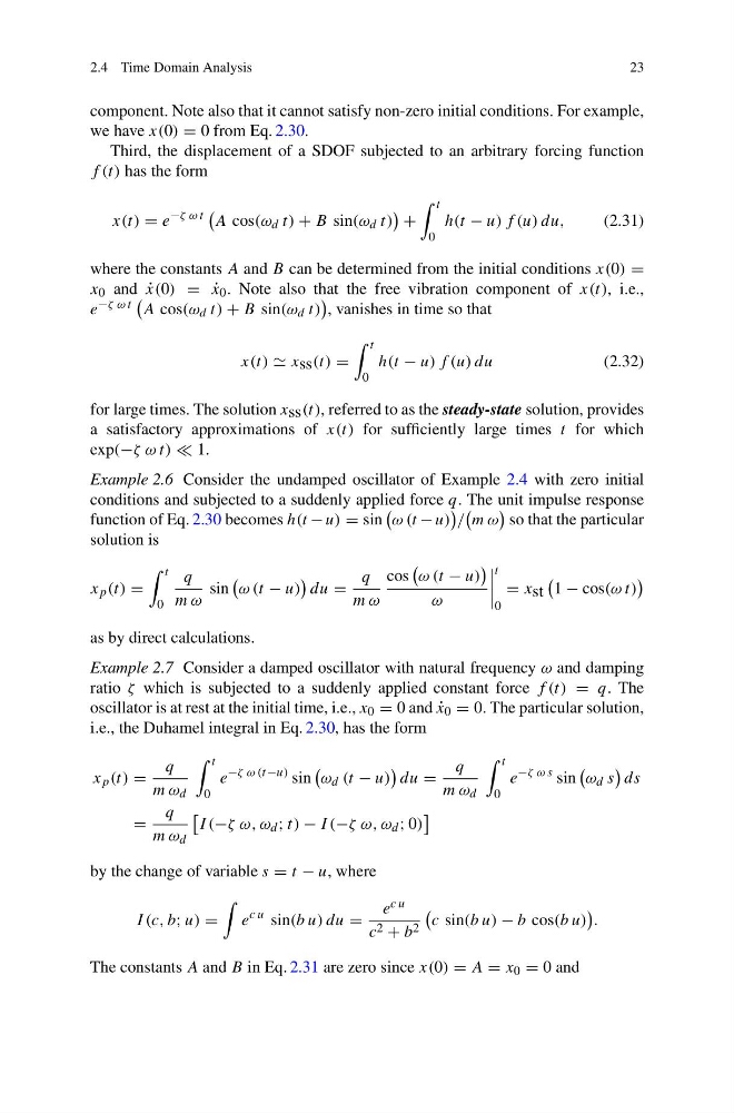
2.4 Time Domain Analysis
23
component. Note also that it cannot satisfy non-zero initial conditions. For example,
we have x(0) = 0 from Eq. 2.30.
Third, the displacement of a SDOF subjected to an arbitrary forcing function
f (t) has the form
x(t) = e
−ζ ω t
A cos(ω d t) + B sin(ω d t)
+
t
0
h(t − u) f (u) du,
(2.31)
where the constants A and B can be determined from the initial conditions x(0) =
x 0 and ˙
x(0) = ˙
x 0 . Note also that the free vibration component of x(t), i.e.,
e −ζ ω t
A cos(ω d t) + B sin(ω d t)
, vanishes in time so that
x(t) x ss (t) =
t
0
h(t − u) f (u) du
(2.32)
for large times. The solution x ss (t), referred to as the steady-state solution, provides
a satisfactory approximations of x(t) for sufficiently large times t for which
exp(−ζ ω t) 1.
Example 2.6 Consider the undamped oscillator of Example 2.4 with zero initial
conditions and subjected to a suddenly applied force q. The unit impulse response
function of Eq. 2.30 becomes h(t − u) = sin
ω (t − u)
/
m ω
so that the particular
solution is
x p (t) =
t
0
q
m ω
sin
ω (t − u)
du =
q
m ω
cos
ω (t − u)
ω
t
0
= x st
1 − cos(ω t)
as by direct calculations.
Example 2.7 Consider a damped oscillator with natural frequency ω and damping
ratio ζ which is subjected to a suddenly applied constant force f (t) = q. The
oscillator is at rest at the initial time, i.e., x 0 = 0 and ˙
x 0 = 0. The particular solution,
i.e., the Duhamel integral in Eq. 2.30, has the form
x p (t) =
q
m ω d
t
0
e
−ζ ω (t−u) sin
ω d (t − u)
du =
q
m ω d
t
0
e
−ζ ω s sin
ω d s
ds
=
q
m ω d
I (−ζ ω, ω d ; t) − I (−ζ ω, ω d ; 0)
by the change of variable s = t − u, where
I (c, b; u) =
e
c u sin(b u) du =
e c u
c 2 + b 2
c sin(b u) − b cos(b u)
.
The constants A and B in Eq. 2.31 are zero since x(0) = A = x 0 = 0 and