

128
5 Continuous Systems
systems, a sum of basis functions {ϕ n (x)} that depend on the system mechanical
properties, topology, and boundary conditions, which are weighted by the timedependent functions {q n (t)}.
5.2.3 Forced Vibration
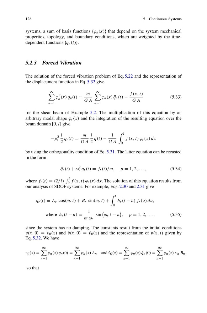
The solution of the forced vibration problem of Eq. 5.22 and the representation of
the displacement function in Eq. 5.32 give
∞
n=1
ϕ
n (x) q n (t) =
m
G A
∞
n=1
ϕ n (x) ¨
q n (t) −
f (x, t)
G A
(5.33)
for the shear beam of Example 5.2. The multiplication of this equation by an
arbitrary modal shape ϕ r (x) and the integration of the resulting equation over the
beam domain [0, l] give
−ρ
2
r
l
2
q r (t) =
m
G A
l
2
¨
q(t) −
1
G A
l
0
f (x, t) ϕ r (x) dx
by using the orthogonality condition of Eq. 5.31. The latter equation can be recasted
in the form
¨
q r (t) + ω
2
r q r (t) = f r (t)/m, p = 1, 2, . . . ,
(5.34)
where f r (t) = (2/l)
l
0 f (x, t) ϕ r (x) dx. The solution of this equation results from
our analysis of SDOF systems. For example, Eqs. 2.30 and 2.31 give
q r (t) = A r cos(ω r t) + B r sin(ω r t) +
t
0
h r (t − u) f r (u) du,
where h r (t − u) =
1
m ω r
sin
ω r t − u
, p = 1, 2, . . . ,
(5.35)
since the system has no damping. The constants result from the initial conditions
v(x, 0) = v 0 (x) and ˙
v(x, 0) = ˙
v 0 (x) and the representation of v(x, t) given by
Eq. 5.32. We have
v 0 (x) =
∞
n=1
ϕ n (x) q n (0) =
∞
n=1
ϕ n (x) A n and ˙
v 0 (x) =
∞
n=1
ϕ n (x) ˙
q n (0) =
∞
n=1
ϕ n (x) ω n B n ,
so that
5 Continuous Systems
systems, a sum of basis functions {ϕ n (x)} that depend on the system mechanical
properties, topology, and boundary conditions, which are weighted by the timedependent functions {q n (t)}.
5.2.3 Forced Vibration
The solution of the forced vibration problem of Eq. 5.22 and the representation of
the displacement function in Eq. 5.32 give
∞
n=1
ϕ
n (x) q n (t) =
m
G A
∞
n=1
ϕ n (x) ¨
q n (t) −
f (x, t)
G A
(5.33)
for the shear beam of Example 5.2. The multiplication of this equation by an
arbitrary modal shape ϕ r (x) and the integration of the resulting equation over the
beam domain [0, l] give
−ρ
2
r
l
2
q r (t) =
m
G A
l
2
¨
q(t) −
1
G A
l
0
f (x, t) ϕ r (x) dx
by using the orthogonality condition of Eq. 5.31. The latter equation can be recasted
in the form
¨
q r (t) + ω
2
r q r (t) = f r (t)/m, p = 1, 2, . . . ,
(5.34)
where f r (t) = (2/l)
l
0 f (x, t) ϕ r (x) dx. The solution of this equation results from
our analysis of SDOF systems. For example, Eqs. 2.30 and 2.31 give
q r (t) = A r cos(ω r t) + B r sin(ω r t) +
t
0
h r (t − u) f r (u) du,
where h r (t − u) =
1
m ω r
sin
ω r t − u
, p = 1, 2, . . . ,
(5.35)
since the system has no damping. The constants result from the initial conditions
v(x, 0) = v 0 (x) and ˙
v(x, 0) = ˙
v 0 (x) and the representation of v(x, t) given by
Eq. 5.32. We have
v 0 (x) =
∞
n=1
ϕ n (x) q n (0) =
∞
n=1
ϕ n (x) A n and ˙
v 0 (x) =
∞
n=1
ϕ n (x) ˙
q n (0) =
∞
n=1
ϕ n (x) ω n B n ,
so that