

5.2 Shear Beams
127
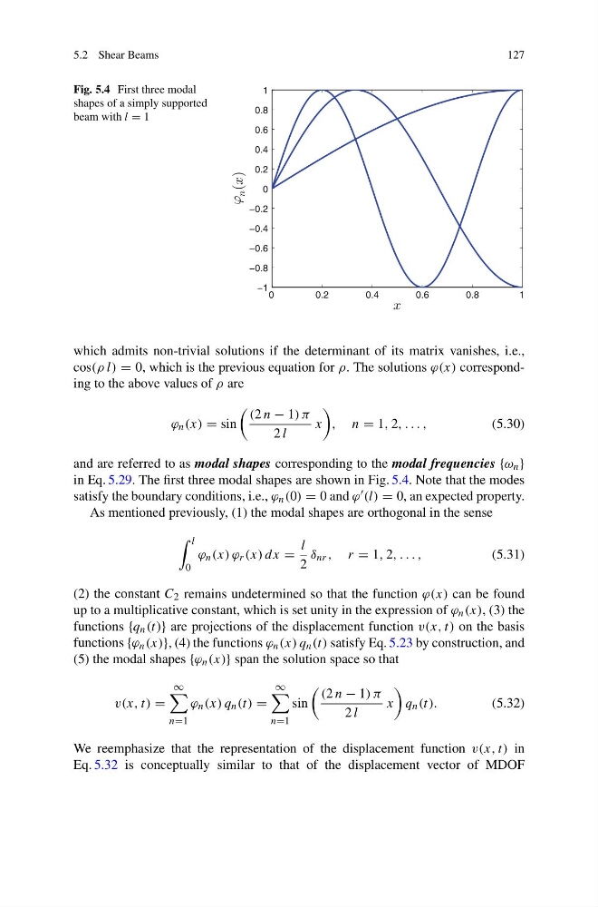
Fig. 5.4 First three modal
shapes of a simply supported
beam with l = 1
0
0.2
0.4
0.6
0.8
1
−1
−0.8
−0.6
−0.4
−0.2
0
0.2
0.4
0.6
0.8
1
x
n (x)
which admits non-trivial solutions if the determinant of its matrix vanishes, i.e.,
cos(ρ l) = 0, which is the previous equation for ρ. The solutions ϕ(x) corresponding to the above values of ρ are
ϕ n (x) = sin
(2 n − 1) π
2 l
x
, n = 1, 2, . . . ,
(5.30)
and are referred to as modal shapes corresponding to the modal frequencies {ω n }
in Eq. 5.29. The first three modal shapes are shown in Fig. 5.4. Note that the modes
satisfy the boundary conditions, i.e., ϕ n (0) = 0 and ϕ (l) = 0, an expected property.
As mentioned previously, (1) the modal shapes are orthogonal in the sense
l
0
ϕ n (x) ϕ r (x) dx =
l
2
δ nr , r = 1, 2, . . . ,
(5.31)
(2) the constant C 2 remains undetermined so that the function ϕ(x) can be found
up to a multiplicative constant, which is set unity in the expression of ϕ n (x), (3) the
functions {q n (t)} are projections of the displacement function v(x, t) on the basis
functions {ϕ n (x)}, (4) the functions ϕ n (x) q n (t) satisfy Eq. 5.23 by construction, and
(5) the modal shapes {ϕ n (x)} span the solution space so that
v(x, t) =
∞
n=1
ϕ n (x) q n (t) =
∞
n=1
sin
(2 n − 1) π
2 l
x
q n (t).
(5.32)
We reemphasize that the representation of the displacement function v(x, t) in
Eq. 5.32 is conceptually similar to that of the displacement vector of MDOF
127
Fig. 5.4 First three modal
shapes of a simply supported
beam with l = 1
0
0.2
0.4
0.6
0.8
1
−1
−0.8
−0.6
−0.4
−0.2
0
0.2
0.4
0.6
0.8
1
x
n (x)
which admits non-trivial solutions if the determinant of its matrix vanishes, i.e.,
cos(ρ l) = 0, which is the previous equation for ρ. The solutions ϕ(x) corresponding to the above values of ρ are
ϕ n (x) = sin
(2 n − 1) π
2 l
x
, n = 1, 2, . . . ,
(5.30)
and are referred to as modal shapes corresponding to the modal frequencies {ω n }
in Eq. 5.29. The first three modal shapes are shown in Fig. 5.4. Note that the modes
satisfy the boundary conditions, i.e., ϕ n (0) = 0 and ϕ (l) = 0, an expected property.
As mentioned previously, (1) the modal shapes are orthogonal in the sense
l
0
ϕ n (x) ϕ r (x) dx =
l
2
δ nr , r = 1, 2, . . . ,
(5.31)
(2) the constant C 2 remains undetermined so that the function ϕ(x) can be found
up to a multiplicative constant, which is set unity in the expression of ϕ n (x), (3) the
functions {q n (t)} are projections of the displacement function v(x, t) on the basis
functions {ϕ n (x)}, (4) the functions ϕ n (x) q n (t) satisfy Eq. 5.23 by construction, and
(5) the modal shapes {ϕ n (x)} span the solution space so that
v(x, t) =
∞
n=1
ϕ n (x) q n (t) =
∞
n=1
sin
(2 n − 1) π
2 l
x
q n (t).
(5.32)
We reemphasize that the representation of the displacement function v(x, t) in
Eq. 5.32 is conceptually similar to that of the displacement vector of MDOF