

5.2 Shear Beams
125
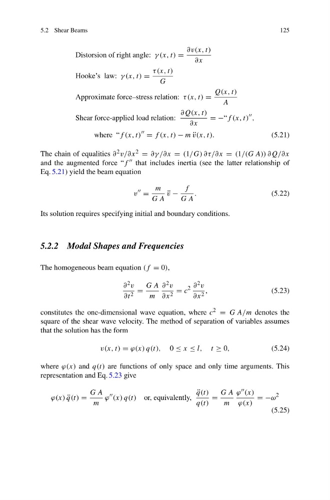
Distorsion of right angle: γ (x, t) =
∂v(x, t)
∂x
Hooke’s law: γ (x, t) =
τ (x, t)
G
Approximate force–stress relation: τ (x, t) =
Q(x, t)
A
Shear force-applied load relation:
∂Q(x, t)
∂x
= −“f (x, t)
,
where “f (x, t)
= f (x, t) − m ¨
v(x, t).
(5.21)
The chain of equalities ∂ 2 v/∂x 2 = ∂γ /∂x = (1/G) ∂τ/∂x = (1/(G A)) ∂Q/∂x
and the augmented force “f that includes inertia (see the latter relationship of
Eq. 5.21) yield the beam equation
v
=
m
G A
¨
v −
f
G A
.
(5.22)
Its solution requires specifying initial and boundary conditions.
5.2.2 Modal Shapes and Frequencies
The homogeneous beam equation (f = 0),
∂ 2 v
∂t 2 =
G A
m
∂ 2 v
∂x 2 = c
2 ∂ 2 v
∂x 2 ,
(5.23)
constitutes the one-dimensional wave equation, where c 2 = G A/m denotes the
square of the shear wave velocity. The method of separation of variables assumes
that the solution has the form
v(x, t) = ϕ(x) q(t), 0 ≤ x ≤ l, t ≥ 0,
(5.24)
where ϕ(x) and q(t) are functions of only space and only time arguments. This
representation and Eq. 5.23 give
ϕ(x) ¨
q(t) =
G A
m
ϕ
(x) q(t) or, equivalently,
¨
q(t)
q(t)
=
G A
m
ϕ (x)
ϕ(x)
= −ω
2
(5.25)
125
Distorsion of right angle: γ (x, t) =
∂v(x, t)
∂x
Hooke’s law: γ (x, t) =
τ (x, t)
G
Approximate force–stress relation: τ (x, t) =
Q(x, t)
A
Shear force-applied load relation:
∂Q(x, t)
∂x
= −“f (x, t)
,
where “f (x, t)
= f (x, t) − m ¨
v(x, t).
(5.21)
The chain of equalities ∂ 2 v/∂x 2 = ∂γ /∂x = (1/G) ∂τ/∂x = (1/(G A)) ∂Q/∂x
and the augmented force “f that includes inertia (see the latter relationship of
Eq. 5.21) yield the beam equation
v
=
m
G A
¨
v −
f
G A
.
(5.22)
Its solution requires specifying initial and boundary conditions.
5.2.2 Modal Shapes and Frequencies
The homogeneous beam equation (f = 0),
∂ 2 v
∂t 2 =
G A
m
∂ 2 v
∂x 2 = c
2 ∂ 2 v
∂x 2 ,
(5.23)
constitutes the one-dimensional wave equation, where c 2 = G A/m denotes the
square of the shear wave velocity. The method of separation of variables assumes
that the solution has the form
v(x, t) = ϕ(x) q(t), 0 ≤ x ≤ l, t ≥ 0,
(5.24)
where ϕ(x) and q(t) are functions of only space and only time arguments. This
representation and Eq. 5.23 give
ϕ(x) ¨
q(t) =
G A
m
ϕ
(x) q(t) or, equivalently,
¨
q(t)
q(t)
=
G A
m
ϕ (x)
ϕ(x)
= −ω
2
(5.25)