

5.1 Flexural Beams
117
∂Q
∂x
= −“f
, where “f
= f − m(x)
∂ 2 v
∂t 2
∂M
∂x
= Q
∂ 2 v
∂x 2 = −
M
E I
∂ 4 v
∂x 4 = −
∂ 2
∂x 2
M
E I
(5.1)
If the stiffness E I is constant, we have
∂ 4 v
∂x 4 =
“f
E I
=
f
E I
−
m(x)
E I
∂ 2 v
∂t 2 .
(5.2)
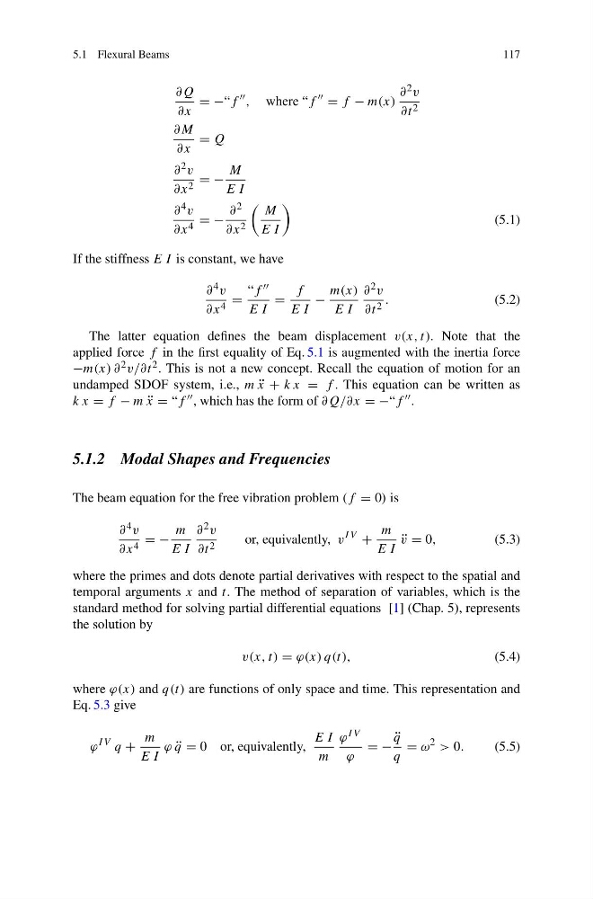
The latter equation defines the beam displacement v(x, t). Note that the
applied force f in the first equality of Eq. 5.1 is augmented with the inertia force
−m(x) ∂ 2 v/∂t 2 . This is not a new concept. Recall the equation of motion for an
undamped SDOF system, i.e., m ¨
x + k x = f . This equation can be written as
k x = f − m ¨
x = “f , which has the form of ∂Q/∂x = −“f .
5.1.2 Modal Shapes and Frequencies
The beam equation for the free vibration problem (f = 0) is
∂ 4 v
∂x 4 = −
m
E I
∂ 2 v
∂t 2
or, equivalently, v
I V
+
m
E I
¨
v = 0,
(5.3)
where the primes and dots denote partial derivatives with respect to the spatial and
temporal arguments x and t. The method of separation of variables, which is the
standard method for solving partial differential equations [1] (Chap. 5), represents
the solution by
v(x, t) = ϕ(x) q(t),
(5.4)
where ϕ(x) and q(t) are functions of only space and time. This representation and
Eq. 5.3 give
ϕ
I V q +
m
E I
ϕ ¨
q = 0 or, equivalently,
E I
m
ϕ I V
ϕ
= −
¨
q
q
= ω
2 > 0.
(5.5)
117
∂Q
∂x
= −“f
, where “f
= f − m(x)
∂ 2 v
∂t 2
∂M
∂x
= Q
∂ 2 v
∂x 2 = −
M
E I
∂ 4 v
∂x 4 = −
∂ 2
∂x 2
M
E I
(5.1)
If the stiffness E I is constant, we have
∂ 4 v
∂x 4 =
“f
E I
=
f
E I
−
m(x)
E I
∂ 2 v
∂t 2 .
(5.2)
The latter equation defines the beam displacement v(x, t). Note that the
applied force f in the first equality of Eq. 5.1 is augmented with the inertia force
−m(x) ∂ 2 v/∂t 2 . This is not a new concept. Recall the equation of motion for an
undamped SDOF system, i.e., m ¨
x + k x = f . This equation can be written as
k x = f − m ¨
x = “f , which has the form of ∂Q/∂x = −“f .
5.1.2 Modal Shapes and Frequencies
The beam equation for the free vibration problem (f = 0) is
∂ 4 v
∂x 4 = −
m
E I
∂ 2 v
∂t 2
or, equivalently, v
I V
+
m
E I
¨
v = 0,
(5.3)
where the primes and dots denote partial derivatives with respect to the spatial and
temporal arguments x and t. The method of separation of variables, which is the
standard method for solving partial differential equations [1] (Chap. 5), represents
the solution by
v(x, t) = ϕ(x) q(t),
(5.4)
where ϕ(x) and q(t) are functions of only space and time. This representation and
Eq. 5.3 give
ϕ
I V q +
m
E I
ϕ ¨
q = 0 or, equivalently,
E I
m
ϕ I V
ϕ
= −
¨
q
q
= ω
2 > 0.
(5.5)