

108
4 Multi-Degree of Freedom (MDOF) Systems
4.6.2 Steady-State Solution: Proportional Damping
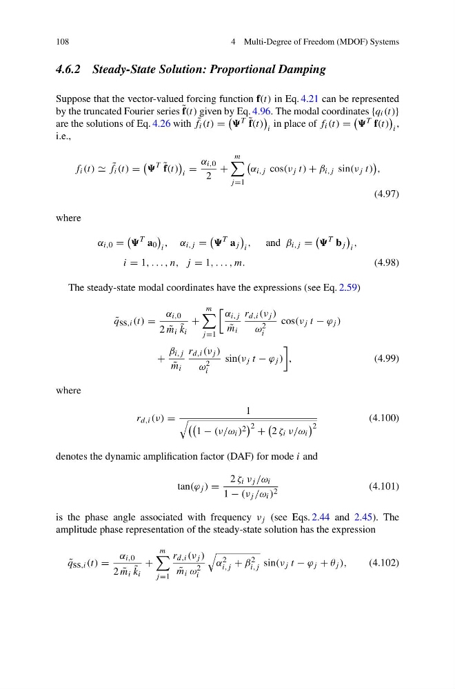
Suppose that the vector-valued forcing function f(t) in Eq. 4.21 can be represented
by the truncated Fourier series ˜ f(t) given by Eq. 4.96. The modal coordinates {q i (t)}
are the solutions of Eq. 4.26 with ˜
f i (t) =
T ˜ f(t)
i
in place of f i (t) =
T f(t)
i
,
i.e.,
f i (t) ˜
f i (t) =
T ˜ f(t)
i
=
α i,0
2
+
m
j =1
α i,j cos(ν j t) + β i,j sin(ν j t)
,
(4.97)
where
α i,0 =
T a 0
i
, α i,j =
T a j
i
, and β i,j =
T b j
i
,
i = 1, . . . , n, j = 1, . . . , m.
(4.98)
The steady-state modal coordinates have the expressions (see Eq. 2.59)
˜
q ss,i (t) =
α i,0
2 ˜
m i ˜
k i
+
m
j =1
α i,j
˜
m i
r d,i (ν j )
ω 2
i
cos(ν j t − ϕ j )
+
β i,j
˜
m i
r d,i (ν j )
ω 2
i
sin(ν j t − ϕ j )
,
(4.99)
where
r d,i (ν) =
1
1 − (ν/ω i ) 2
2 +
2 ζ i ν/ω i
2
(4.100)
denotes the dynamic amplification factor (DAF) for mode i and
tan(ϕ j ) =
2 ζ i ν j /ω i
1 − (ν j /ω i ) 2
(4.101)
is the phase angle associated with frequency ν j (see Eqs. 2.44 and 2.45). The
amplitude phase representation of the steady-state solution has the expression
˜
q ss,i (t) =
α i,0
2 ˜
m i ˜
k i
+
m
j =1
r d,i (ν j )
˜
m i ω 2
i
α 2
i,j + β 2
i,j sin(ν j t − ϕ j + θ j ),
(4.102)
4 Multi-Degree of Freedom (MDOF) Systems
4.6.2 Steady-State Solution: Proportional Damping
Suppose that the vector-valued forcing function f(t) in Eq. 4.21 can be represented
by the truncated Fourier series ˜ f(t) given by Eq. 4.96. The modal coordinates {q i (t)}
are the solutions of Eq. 4.26 with ˜
f i (t) =
T ˜ f(t)
i
in place of f i (t) =
T f(t)
i
,
i.e.,
f i (t) ˜
f i (t) =
T ˜ f(t)
i
=
α i,0
2
+
m
j =1
α i,j cos(ν j t) + β i,j sin(ν j t)
,
(4.97)
where
α i,0 =
T a 0
i
, α i,j =
T a j
i
, and β i,j =
T b j
i
,
i = 1, . . . , n, j = 1, . . . , m.
(4.98)
The steady-state modal coordinates have the expressions (see Eq. 2.59)
˜
q ss,i (t) =
α i,0
2 ˜
m i ˜
k i
+
m
j =1
α i,j
˜
m i
r d,i (ν j )
ω 2
i
cos(ν j t − ϕ j )
+
β i,j
˜
m i
r d,i (ν j )
ω 2
i
sin(ν j t − ϕ j )
,
(4.99)
where
r d,i (ν) =
1
1 − (ν/ω i ) 2
2 +
2 ζ i ν/ω i
2
(4.100)
denotes the dynamic amplification factor (DAF) for mode i and
tan(ϕ j ) =
2 ζ i ν j /ω i
1 − (ν j /ω i ) 2
(4.101)
is the phase angle associated with frequency ν j (see Eqs. 2.44 and 2.45). The
amplitude phase representation of the steady-state solution has the expression
˜
q ss,i (t) =
α i,0
2 ˜
m i ˜
k i
+
m
j =1
r d,i (ν j )
˜
m i ω 2
i
α 2
i,j + β 2
i,j sin(ν j t − ϕ j + θ j ),
(4.102)