

104
4 Multi-Degree of Freedom (MDOF) Systems
¨
x + 2 ζ ω ˙
x + ω
2 x = 1, t ≥ 0,
with zero initial conditions, and has the expression (see Example 2.5)
x(t) =
1
ω 2
e
−ζ ω t
−
ζ
1 − ζ 2
sin(ω d t) − cos(ω d t)
+ 1
.
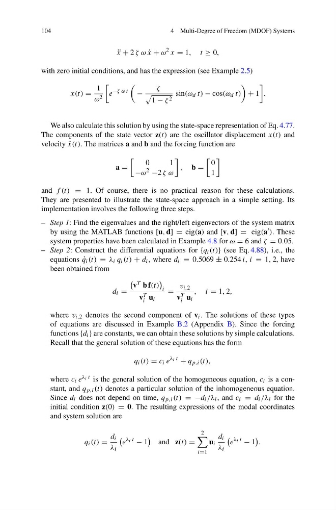
We also calculate this solution by using the state-space representation of Eq. 4.77.
The components of the state vector z(t) are the oscillator displacement x(t) and
velocity ˙
x(t). The matrices a and b and the forcing function are
a =
0
1
−ω 2 −2 ζ ω
, b =
0
1
and f (t) = 1. Of course, there is no practical reason for these calculations.
They are presented to illustrate the state-space approach in a simple setting. Its
implementation involves the following three steps.
– Step 1: Find the eigenvalues and the right/left eigenvectors of the system matrix
by using the MATLAB functions [u, d] = eig(a) and [v, d] = eig(a ). These
system properties have been calculated in Example 4.8 for ω = 6 and ζ = 0.05.
– Step 2: Construct the differential equations for {q i (t)} (see Eq. 4.88), i.e., the
equations ˙
q i (t) = λ i q i (t) + d i , where d i = 0.5069 ± 0.254 i, i = 1, 2, have
been obtained from
d i =
v T b f(t)
i
v T
i u i
=
v i,2
v T
i u i
, i = 1, 2,
where v i,2 denotes the second component of v i . The solutions of these types
of equations are discussed in Example B.2 (Appendix B). Since the forcing
functions {d i } are constants, we can obtain these solutions by simple calculations.
Recall that the general solution of these equations has the form
q i (t) = c i e
λ i t
+ q p,i (t),
where c i e λ i t is the general solution of the homogeneous equation, c i is a constant, and q p,i (t) denotes a particular solution of the inhomogeneous equation.
Since d i does not depend on time, q p,i (t) = −d i /λ i , and c i = d i /λ i for the
initial condition z(0) = 0. The resulting expressions of the modal coordinates
and system solution are
q i (t) =
d i
λ i
e
λ i t
− 1
and z(t) =
2
i=1
u i
d i
λ i
e
λ i t
− 1
.
4 Multi-Degree of Freedom (MDOF) Systems
¨
x + 2 ζ ω ˙
x + ω
2 x = 1, t ≥ 0,
with zero initial conditions, and has the expression (see Example 2.5)
x(t) =
1
ω 2
e
−ζ ω t
−
ζ
1 − ζ 2
sin(ω d t) − cos(ω d t)
+ 1
.
We also calculate this solution by using the state-space representation of Eq. 4.77.
The components of the state vector z(t) are the oscillator displacement x(t) and
velocity ˙
x(t). The matrices a and b and the forcing function are
a =
0
1
−ω 2 −2 ζ ω
, b =
0
1
and f (t) = 1. Of course, there is no practical reason for these calculations.
They are presented to illustrate the state-space approach in a simple setting. Its
implementation involves the following three steps.
– Step 1: Find the eigenvalues and the right/left eigenvectors of the system matrix
by using the MATLAB functions [u, d] = eig(a) and [v, d] = eig(a ). These
system properties have been calculated in Example 4.8 for ω = 6 and ζ = 0.05.
– Step 2: Construct the differential equations for {q i (t)} (see Eq. 4.88), i.e., the
equations ˙
q i (t) = λ i q i (t) + d i , where d i = 0.5069 ± 0.254 i, i = 1, 2, have
been obtained from
d i =
v T b f(t)
i
v T
i u i
=
v i,2
v T
i u i
, i = 1, 2,
where v i,2 denotes the second component of v i . The solutions of these types
of equations are discussed in Example B.2 (Appendix B). Since the forcing
functions {d i } are constants, we can obtain these solutions by simple calculations.
Recall that the general solution of these equations has the form
q i (t) = c i e
λ i t
+ q p,i (t),
where c i e λ i t is the general solution of the homogeneous equation, c i is a constant, and q p,i (t) denotes a particular solution of the inhomogeneous equation.
Since d i does not depend on time, q p,i (t) = −d i /λ i , and c i = d i /λ i for the
initial condition z(0) = 0. The resulting expressions of the modal coordinates
and system solution are
q i (t) =
d i
λ i
e
λ i t
− 1
and z(t) =
2
i=1
u i
d i
λ i
e
λ i t
− 1
.