

4.5 Time Domain Analysis: Non-proportional Damping
101
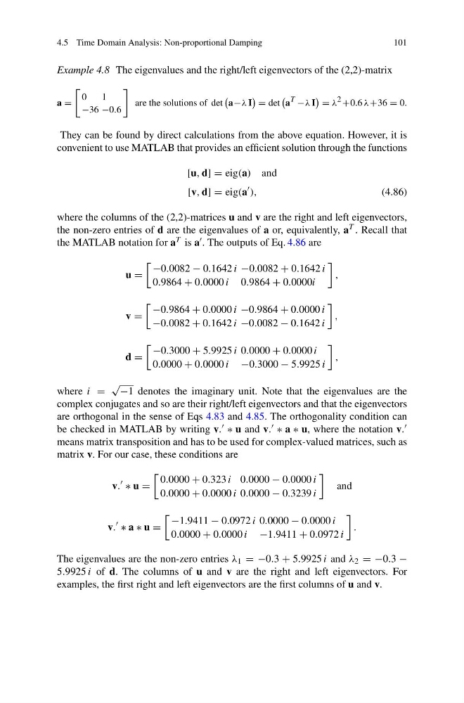
Example 4.8 The eigenvalues and the right/left eigenvectors of the (2,2)-matrix
a =
0
1
−36 −0.6
are the solutions of det
a−λ I
= det
a T −λ I
= λ 2 +0.6 λ+36 = 0.
They can be found by direct calculations from the above equation. However, it is
convenient to use MATLAB that provides an efficient solution through the functions
[u, d] = eig(a) and
[v, d] = eig(a
),
(4.86)
where the columns of the (2,2)-matrices u and v are the right and left eigenvectors,
the non-zero entries of d are the eigenvalues of a or, equivalently, a T . Recall that
the MATLAB notation for a T is a . The outputs of Eq. 4.86 are
u =
−0.0082 − 0.1642 i −0.0082 + 0.1642 i
0.9864 + 0.0000 i 0.9864 + 0.0000i
,
v =
−0.9864 + 0.0000 i −0.9864 + 0.0000 i
−0.0082 + 0.1642 i −0.0082 − 0.1642 i
,
d =
−0.3000 + 5.9925 i 0.0000 + 0.0000 i
0.0000 + 0.0000 i −0.3000 − 5.9925 i
,
where i =
√ −1 denotes the imaginary unit. Note that the eigenvalues are the
complex conjugates and so are their right/left eigenvectors and that the eigenvectors
are orthogonal in the sense of Eqs 4.83 and 4.85. The orthogonality condition can
be checked in MATLAB by writing v. ∗ u and v. ∗ a ∗ u, where the notation v.
means matrix transposition and has to be used for complex-valued matrices, such as
matrix v. For our case, these conditions are
v.
∗ u =
0.0000 + 0.323 i 0.0000 − 0.0000 i
0.0000 + 0.0000 i 0.0000 − 0.3239 i
and
v.
∗ a ∗ u =
−1.9411 − 0.0972 i 0.0000 − 0.0000 i
0.0000 + 0.0000 i −1.9411 + 0.0972 i
.
The eigenvalues are the non-zero entries λ 1 = −0.3 + 5.9925 i and λ 2 = −0.3 −
5.9925 i of d. The columns of u and v are the right and left eigenvectors. For
examples, the first right and left eigenvectors are the first columns of u and v.
101
Example 4.8 The eigenvalues and the right/left eigenvectors of the (2,2)-matrix
a =
0
1
−36 −0.6
are the solutions of det
a−λ I
= det
a T −λ I
= λ 2 +0.6 λ+36 = 0.
They can be found by direct calculations from the above equation. However, it is
convenient to use MATLAB that provides an efficient solution through the functions
[u, d] = eig(a) and
[v, d] = eig(a
),
(4.86)
where the columns of the (2,2)-matrices u and v are the right and left eigenvectors,
the non-zero entries of d are the eigenvalues of a or, equivalently, a T . Recall that
the MATLAB notation for a T is a . The outputs of Eq. 4.86 are
u =
−0.0082 − 0.1642 i −0.0082 + 0.1642 i
0.9864 + 0.0000 i 0.9864 + 0.0000i
,
v =
−0.9864 + 0.0000 i −0.9864 + 0.0000 i
−0.0082 + 0.1642 i −0.0082 − 0.1642 i
,
d =
−0.3000 + 5.9925 i 0.0000 + 0.0000 i
0.0000 + 0.0000 i −0.3000 − 5.9925 i
,
where i =
√ −1 denotes the imaginary unit. Note that the eigenvalues are the
complex conjugates and so are their right/left eigenvectors and that the eigenvectors
are orthogonal in the sense of Eqs 4.83 and 4.85. The orthogonality condition can
be checked in MATLAB by writing v. ∗ u and v. ∗ a ∗ u, where the notation v.
means matrix transposition and has to be used for complex-valued matrices, such as
matrix v. For our case, these conditions are
v.
∗ u =
0.0000 + 0.323 i 0.0000 − 0.0000 i
0.0000 + 0.0000 i 0.0000 − 0.3239 i
and
v.
∗ a ∗ u =
−1.9411 − 0.0972 i 0.0000 − 0.0000 i
0.0000 + 0.0000 i −1.9411 + 0.0972 i
.
The eigenvalues are the non-zero entries λ 1 = −0.3 + 5.9925 i and λ 2 = −0.3 −
5.9925 i of d. The columns of u and v are the right and left eigenvectors. For
examples, the first right and left eigenvectors are the first columns of u and v.