

2 On Normalization Functions and ϕ-Families of Probability Distributions
23
0
1
2
3
4
5
0
10
20
30
40
50
60
70
80
90
100
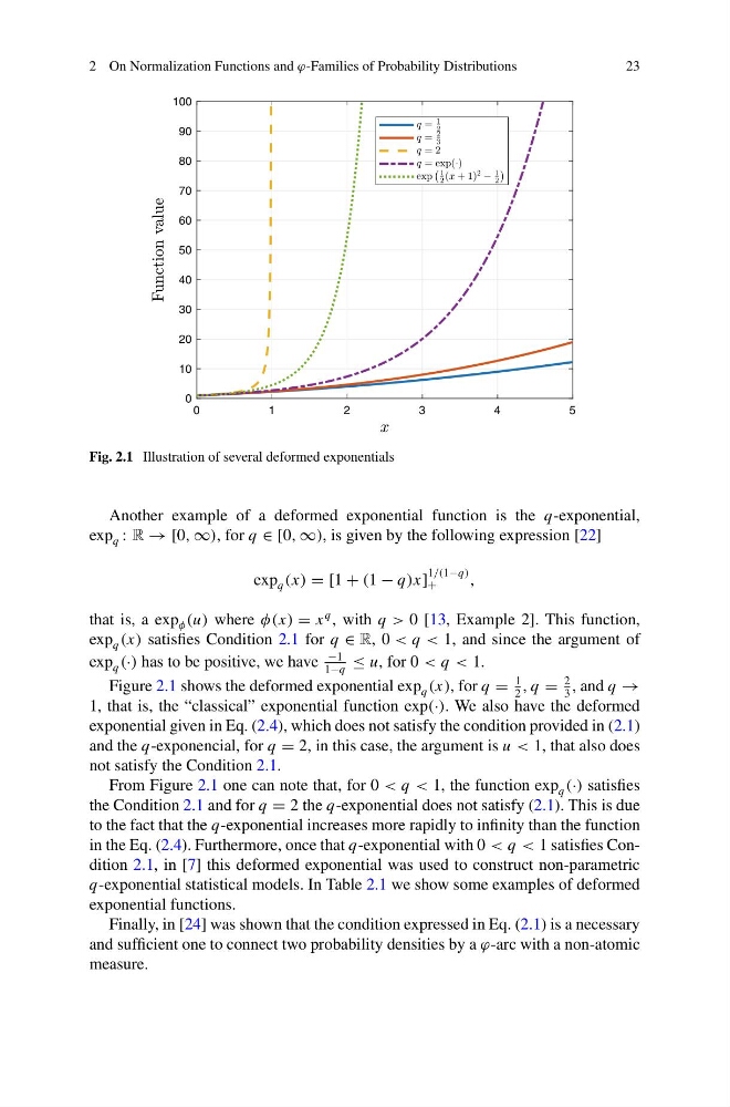
Fig. 2.1 Illustration of several deformed exponentials
Another example of a deformed exponential function is the q-exponential,
exp q : R → [0, ∞), for q ∈ [0, ∞), is given by the following expression [22]
exp q (x) = [1 + (1 − q)x]
1/(1−q)
+
,
that is, a exp φ (u) where φ(x) = x
q , with q > 0 [13, Example 2]. This function,
exp q (x) satisfies Condition 2.1 for q ∈ R, 0 < q < 1, and since the argument of
exp q (·) has to be positive, we have
−1
1−q
≤ u, for 0 < q < 1.
Figure 2.1 shows the deformed exponential exp q (x), for q =
1
2
, q =
2
3
, and q →
1, that is, the “classical” exponential function exp(·). We also have the deformed
exponential given in Eq. (2.4), which does not satisfy the condition provided in (2.1)
and the q-exponencial, for q = 2, in this case, the argument is u < 1, that also does
not satisfy the Condition 2.1.
From Figure 2.1 one can note that, for 0 < q < 1, the function exp q (·) satisfies
the Condition 2.1 and for q = 2 the q-exponential does not satisfy (2.1). This is due
to the fact that the q-exponential increases more rapidly to infinity than the function
in the Eq. (2.4). Furthermore, once that q-exponential with 0 < q < 1 satisfies Condition 2.1, in [7] this deformed exponential was used to construct non-parametric
q-exponential statistical models. In Table 2.1 we show some examples of deformed
exponential functions.
Finally, in [24] was shown that the condition expressed in Eq. (2.1) is a necessary
and sufficient one to connect two probability densities by a ϕ-arc with a non-atomic
measure.
23
0
1
2
3
4
5
0
10
20
30
40
50
60
70
80
90
100
Fig. 2.1 Illustration of several deformed exponentials
Another example of a deformed exponential function is the q-exponential,
exp q : R → [0, ∞), for q ∈ [0, ∞), is given by the following expression [22]
exp q (x) = [1 + (1 − q)x]
1/(1−q)
+
,
that is, a exp φ (u) where φ(x) = x
q , with q > 0 [13, Example 2]. This function,
exp q (x) satisfies Condition 2.1 for q ∈ R, 0 < q < 1, and since the argument of
exp q (·) has to be positive, we have
−1
1−q
≤ u, for 0 < q < 1.
Figure 2.1 shows the deformed exponential exp q (x), for q =
1
2
, q =
2
3
, and q →
1, that is, the “classical” exponential function exp(·). We also have the deformed
exponential given in Eq. (2.4), which does not satisfy the condition provided in (2.1)
and the q-exponencial, for q = 2, in this case, the argument is u < 1, that also does
not satisfy the Condition 2.1.
From Figure 2.1 one can note that, for 0 < q < 1, the function exp q (·) satisfies
the Condition 2.1 and for q = 2 the q-exponential does not satisfy (2.1). This is due
to the fact that the q-exponential increases more rapidly to infinity than the function
in the Eq. (2.4). Furthermore, once that q-exponential with 0 < q < 1 satisfies Condition 2.1, in [7] this deformed exponential was used to construct non-parametric
q-exponential statistical models. In Table 2.1 we show some examples of deformed
exponential functions.
Finally, in [24] was shown that the condition expressed in Eq. (2.1) is a necessary
and sufficient one to connect two probability densities by a ϕ-arc with a non-atomic
measure.