

22
L. H. F. de Andrade et al.
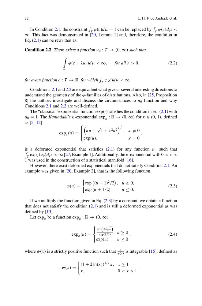
In Condition 2.1, the constraint
T ϕ(c)dμ = 1 can be replaced by
T ϕ(c)dμ <
∞. This fact was demonstrated in [20, Lemma 1] and, therefore, the condition in
Eq. (2.1) can be rewritten as:
Condition 2.2 There exists a function u 0 : T → (0, ∞) such that
T
ϕ(c + λu 0 )dμ < ∞,
for all λ > 0,
(2.2)
for every function c : T → R, for which
T ϕ(c)dμ < ∞.
Conditions 2.1 and 2.2 are equivalent what give us several interesting directions to
understand the geometry of the ϕ-families of distributions. Also, in [25, Proposition
8] the authors investigate and discuss the circumstances to u 0 function and why
Conditions 2.1 and 2.2 are well-defined.
The “classical” exponential function exp(·) satisfies the condition in Eq. (2.1) with
u 0 = 1. The Kaniadaki’s κ-exponential exp κ : R → (0, ∞) for κ ∈ (0, 1), defined
as [5, 12]
exp κ (u) =
⎧
⎨
⎩
κu +
√
1 + κ 2 u 2
1
κ , κ = 0
exp(u),
κ = 0
,
is a deformed exponential that satisfies (2.1) for any function u 0 such that
T exp κ (u 0 )dμ < ∞ [27, Example 1]. Additionally, the κ-exponential with 0 < κ <
1 was used in the construction of a statistical manifold [16].
However, there exist deformed exponentials that do not satisfy Condition 2.1. An
example was given in [20, Example 2], that is the following function,
ϕ(u) =
exp
(u + 1)
2
/2
, u ≥ 0,
exp (u + 1/2) ,
u ≤ 0.
(2.3)
If we multiply the function given in Eq. (2.3) by a constant, we obtain a function
that does not satisfy the condition (2.1) and is still a deformed exponential as was
defined by [13].
Let exp φ be a function exp φ : R → (0, ∞)
exp φ (u) =
⎧
⎨
⎩
exp
(u+1) 2
2
exp(1/2)
u ≥ 0
exp(u)
u ≤ 0
,
(2.4)
where φ(x) is a strictly positive function such that
1
φ(x)
is integrable [15], defined as
φ(x) =
(1 + 2 ln(x))
1/2 x, x ≥ 1
x,
0 < x ≤ 1
.
L. H. F. de Andrade et al.
In Condition 2.1, the constraint
T ϕ(c)dμ = 1 can be replaced by
T ϕ(c)dμ <
∞. This fact was demonstrated in [20, Lemma 1] and, therefore, the condition in
Eq. (2.1) can be rewritten as:
Condition 2.2 There exists a function u 0 : T → (0, ∞) such that
T
ϕ(c + λu 0 )dμ < ∞,
for all λ > 0,
(2.2)
for every function c : T → R, for which
T ϕ(c)dμ < ∞.
Conditions 2.1 and 2.2 are equivalent what give us several interesting directions to
understand the geometry of the ϕ-families of distributions. Also, in [25, Proposition
8] the authors investigate and discuss the circumstances to u 0 function and why
Conditions 2.1 and 2.2 are well-defined.
The “classical” exponential function exp(·) satisfies the condition in Eq. (2.1) with
u 0 = 1. The Kaniadaki’s κ-exponential exp κ : R → (0, ∞) for κ ∈ (0, 1), defined
as [5, 12]
exp κ (u) =
⎧
⎨
⎩
κu +
√
1 + κ 2 u 2
1
κ , κ = 0
exp(u),
κ = 0
,
is a deformed exponential that satisfies (2.1) for any function u 0 such that
T exp κ (u 0 )dμ < ∞ [27, Example 1]. Additionally, the κ-exponential with 0 < κ <
1 was used in the construction of a statistical manifold [16].
However, there exist deformed exponentials that do not satisfy Condition 2.1. An
example was given in [20, Example 2], that is the following function,
ϕ(u) =
exp
(u + 1)
2
/2
, u ≥ 0,
exp (u + 1/2) ,
u ≤ 0.
(2.3)
If we multiply the function given in Eq. (2.3) by a constant, we obtain a function
that does not satisfy the condition (2.1) and is still a deformed exponential as was
defined by [13].
Let exp φ be a function exp φ : R → (0, ∞)
exp φ (u) =
⎧
⎨
⎩
exp
(u+1) 2
2
exp(1/2)
u ≥ 0
exp(u)
u ≤ 0
,
(2.4)
where φ(x) is a strictly positive function such that
1
φ(x)
is integrable [15], defined as
φ(x) =
(1 + 2 ln(x))
1/2 x, x ≥ 1
x,
0 < x ≤ 1
.