

232
A. Cole and G. Shiu
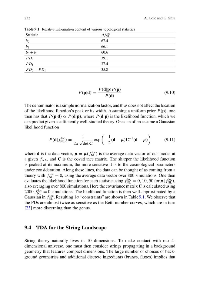
Table 9.1 Relative information content of various topological statistics
Statistic
Δf loc
NL
b 0
67.4
b 1
66.1
b 0 + b 1
60.6
P D 0
39.1
P D 1
37.4
P D 0 + P D 1
35.8
P(p|d) =
P(d|p)P(p)
P(d)
(9.10)
The denominator is a simple normalization factor, and thus does not affect the location
of the likelihood function’s peak or its width. Assuming a uniform prior P(p), one
then has that P(p|d) ∝ P(d|p), where P(d|p) is the likelihood function, which we
can predict given a sufficiently well-studied theory. One can often assume a Gaussian
likelihood function
P(d| f
loc
NL ) =
1
2π
√
det C
exp
−
1
2
(d − µ)C
−1
(d − µ)
(9.11)
where d is the data vector, µ = µ( f
loc
NL ) is the average data vector of our model at
a given f N L , and C is the covariance matrix. The sharper the likelihood function
is peaked at its maximum, the more sensitive it is to the cosmological parameters
under consideration. Along these lines, the data can be thought of as coming from a
theory with f
loc
NL = 0, using the average data vector over 800 simulations. One then
evaluates the likelihood function for each statistic using f
loc
NL = 0, 10, 50 for µ( f
loc
NL ),
also averaging over 800 simulations. Here the covariance matrix C is calculated using
2000 f
loc
NL = 0 simulations. The likelihood function is then well-approximated by a
Gaussian in f
loc
NL . Resulting 1σ “constraints” are shown in Table 9.1. We observe that
the PDs are almost twice as sensitive as the Betti number curves, which are in turn
[23] more discerning than the genus.
9.4 TDA for the String Landscape
String theory naturally lives in 10 dimensions. To make contact with our 4dimensional universe, one must then consider strings propagating in a background
geometry that features compact dimensions. The large number of choices of background geometries and additional discrete ingredients (branes, fluxes) implies that
A. Cole and G. Shiu
Table 9.1 Relative information content of various topological statistics
Statistic
Δf loc
NL
b 0
67.4
b 1
66.1
b 0 + b 1
60.6
P D 0
39.1
P D 1
37.4
P D 0 + P D 1
35.8
P(p|d) =
P(d|p)P(p)
P(d)
(9.10)
The denominator is a simple normalization factor, and thus does not affect the location
of the likelihood function’s peak or its width. Assuming a uniform prior P(p), one
then has that P(p|d) ∝ P(d|p), where P(d|p) is the likelihood function, which we
can predict given a sufficiently well-studied theory. One can often assume a Gaussian
likelihood function
P(d| f
loc
NL ) =
1
2π
√
det C
exp
−
1
2
(d − µ)C
−1
(d − µ)
(9.11)
where d is the data vector, µ = µ( f
loc
NL ) is the average data vector of our model at
a given f N L , and C is the covariance matrix. The sharper the likelihood function
is peaked at its maximum, the more sensitive it is to the cosmological parameters
under consideration. Along these lines, the data can be thought of as coming from a
theory with f
loc
NL = 0, using the average data vector over 800 simulations. One then
evaluates the likelihood function for each statistic using f
loc
NL = 0, 10, 50 for µ( f
loc
NL ),
also averaging over 800 simulations. Here the covariance matrix C is calculated using
2000 f
loc
NL = 0 simulations. The likelihood function is then well-approximated by a
Gaussian in f
loc
NL . Resulting 1σ “constraints” are shown in Table 9.1. We observe that
the PDs are almost twice as sensitive as the Betti number curves, which are in turn
[23] more discerning than the genus.
9.4 TDA for the String Landscape
String theory naturally lives in 10 dimensions. To make contact with our 4dimensional universe, one must then consider strings propagating in a background
geometry that features compact dimensions. The large number of choices of background geometries and additional discrete ingredients (branes, fluxes) implies that