

9 Towards the “Shape” of Cosmological Observables and the String …
231
9.3.2.1 Local Non-Gaussianity
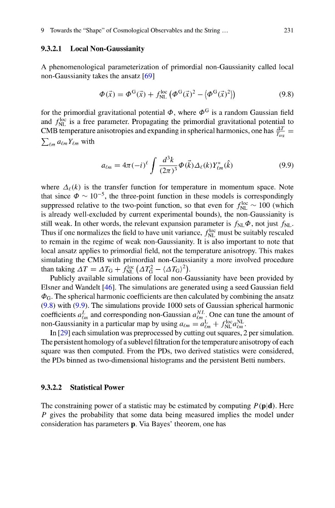
A phenomenological parameterization of primordial non-Gaussianity called local
non-Gaussianity takes the ansatz [69]
Φ( x) = Φ
G
( x) + f
loc
NL
Φ
G
( x)
2
−
Φ
G
( x)
2
(9.8)
for the primordial gravitational potential Φ, where Φ
G is a random Gaussian field
and f
loc
NL is a free parameter. Propagating the primordial gravitational potential to
CMB temperature anisotropies and expanding in spherical harmonics, one has
ΔT
T avg
=
m a m Y m with
a m = 4π(−i)
d
3 k
(2π) 3 Φ(
k)Δ (k)Y
∗
m ( ˆ
k)
(9.9)
where Δ (k) is the transfer function for temperature in momentum space. Note
that since Φ ∼ 10
−5 , the three-point function in these models is correspondingly
suppressed relative to the two-point function, so that even for f
loc
NL ∼ 100 (which
is already well-excluded by current experimental bounds), the non-Gaussianity is
still weak. In other words, the relevant expansion parameter is f NL Φ, not just f NL .
Thus if one normalizes the field to have unit variance, f
loc
NL must be suitably rescaled
to remain in the regime of weak non-Gaussianity. It is also important to note that
local ansatz applies to primordial field, not the temperature anisotropy. This makes
simulating the CMB with primordial non-Gaussianity a more involved procedure
than taking ΔT = ΔT G + f
loc
NL
ΔT
2
G − ΔT G
2
.
Publicly available simulations of local non-Gaussianity have been provided by
Elsner and Wandelt [46]. The simulations are generated using a seed Gaussian field
Φ G . The spherical harmonic coefficients are then calculated by combining the ansatz
(9.8) with (9.9). The simulations provide 1000 sets of Gaussian spherical harmonic
coefficients a
L
m and corresponding non-Gaussian a
N L
m . One can tune the amount of
non-Gaussianity in a particular map by using a m = a
L
m + f
loc
NL a
NL
m .
In [29] each simulation was preprocessed by cutting out squares, 2 per simulation.
The persistent homology of a sublevel filtration for the temperature anisotropy of each
square was then computed. From the PDs, two derived statistics were considered,
the PDs binned as two-dimensional histograms and the persistent Betti numbers.
9.3.2.2 Statistical Power
The constraining power of a statistic may be estimated by computing P(p|d). Here
P gives the probability that some data being measured implies the model under
consideration has parameters p. Via Bayes’ theorem, one has
231
9.3.2.1 Local Non-Gaussianity
A phenomenological parameterization of primordial non-Gaussianity called local
non-Gaussianity takes the ansatz [69]
Φ( x) = Φ
G
( x) + f
loc
NL
Φ
G
( x)
2
−
Φ
G
( x)
2
(9.8)
for the primordial gravitational potential Φ, where Φ
G is a random Gaussian field
and f
loc
NL is a free parameter. Propagating the primordial gravitational potential to
CMB temperature anisotropies and expanding in spherical harmonics, one has
ΔT
T avg
=
m a m Y m with
a m = 4π(−i)
d
3 k
(2π) 3 Φ(
k)Δ (k)Y
∗
m ( ˆ
k)
(9.9)
where Δ (k) is the transfer function for temperature in momentum space. Note
that since Φ ∼ 10
−5 , the three-point function in these models is correspondingly
suppressed relative to the two-point function, so that even for f
loc
NL ∼ 100 (which
is already well-excluded by current experimental bounds), the non-Gaussianity is
still weak. In other words, the relevant expansion parameter is f NL Φ, not just f NL .
Thus if one normalizes the field to have unit variance, f
loc
NL must be suitably rescaled
to remain in the regime of weak non-Gaussianity. It is also important to note that
local ansatz applies to primordial field, not the temperature anisotropy. This makes
simulating the CMB with primordial non-Gaussianity a more involved procedure
than taking ΔT = ΔT G + f
loc
NL
ΔT
2
G − ΔT G
2
.
Publicly available simulations of local non-Gaussianity have been provided by
Elsner and Wandelt [46]. The simulations are generated using a seed Gaussian field
Φ G . The spherical harmonic coefficients are then calculated by combining the ansatz
(9.8) with (9.9). The simulations provide 1000 sets of Gaussian spherical harmonic
coefficients a
L
m and corresponding non-Gaussian a
N L
m . One can tune the amount of
non-Gaussianity in a particular map by using a m = a
L
m + f
loc
NL a
NL
m .
In [29] each simulation was preprocessed by cutting out squares, 2 per simulation.
The persistent homology of a sublevel filtration for the temperature anisotropy of each
square was then computed. From the PDs, two derived statistics were considered,
the PDs binned as two-dimensional histograms and the persistent Betti numbers.
9.3.2.2 Statistical Power
The constraining power of a statistic may be estimated by computing P(p|d). Here
P gives the probability that some data being measured implies the model under
consideration has parameters p. Via Bayes’ theorem, one has