

222
A. Cole and G. Shiu
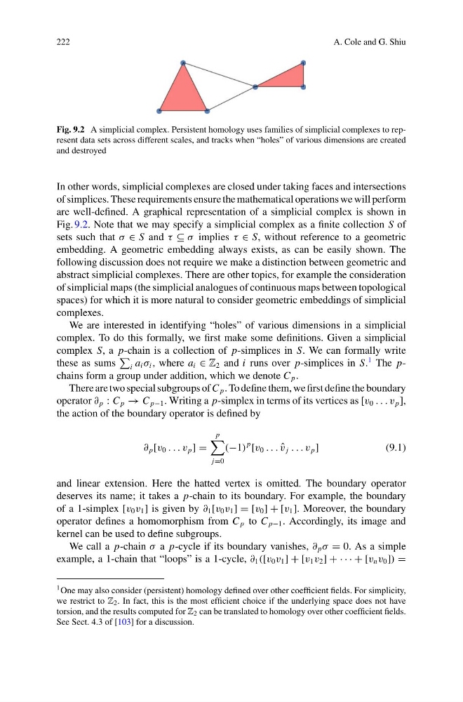
Fig. 9.2 A simplicial complex. Persistent homology uses families of simplicial complexes to represent data sets across different scales, and tracks when “holes” of various dimensions are created
and destroyed
In other words, simplicial complexes are closed under taking faces and intersections
of simplices. These requirements ensure the mathematical operations we will perform
are well-defined. A graphical representation of a simplicial complex is shown in
Fig. 9.2. Note that we may specify a simplicial complex as a finite collection S of
sets such that σ ∈ S and τ ⊆ σ implies τ ∈ S, without reference to a geometric
embedding. A geometric embedding always exists, as can be easily shown. The
following discussion does not require we make a distinction between geometric and
abstract simplicial complexes. There are other topics, for example the consideration
of simplicial maps (the simplicial analogues of continuous maps between topological
spaces) for which it is more natural to consider geometric embeddings of simplicial
complexes.
We are interested in identifying “holes” of various dimensions in a simplicial
complex. To do this formally, we first make some definitions. Given a simplicial
complex S, a p-chain is a collection of p-simplices in S. We can formally write
these as sums
i a i σ i , where a i ∈ Z 2 and i runs over p-simplices in S.
1 The pchains form a group under addition, which we denote C p .
There are two special subgroups of C p . To define them, we first define the boundary
operator ∂ p : C p → C p−1 . Writing a p-simplex in terms of its vertices as [v 0 . . . v p ],
the action of the boundary operator is defined by
∂ p [v 0 . . . v p ] =
p
j=0
(−1)
p
[v 0 . . . ˆ
v j . . . v p ]
(9.1)
and linear extension. Here the hatted vertex is omitted. The boundary operator
deserves its name; it takes a p-chain to its boundary. For example, the boundary
of a 1-simplex [v 0 v 1 ] is given by ∂ 1 [v 0 v 1 ] = [v 0 ] + [v 1 ]. Moreover, the boundary
operator defines a homomorphism from C p to C p−1 . Accordingly, its image and
kernel can be used to define subgroups.
We call a p-chain σ a p-cycle if its boundary vanishes, ∂ p σ = 0. As a simple
example, a 1-chain that “loops” is a 1-cycle, ∂ 1 ([v 0 v 1 ] + [v 1 v 2 ] + · · · + [v n v 0 ]) =
1 One may also consider (persistent) homology defined over other coefficient fields. For simplicity,
we restrict to Z 2 . In fact, this is the most efficient choice if the underlying space does not have
torsion, and the results computed for Z 2 can be translated to homology over other coefficient fields.
See Sect. 4.3 of [103] for a discussion.
A. Cole and G. Shiu
Fig. 9.2 A simplicial complex. Persistent homology uses families of simplicial complexes to represent data sets across different scales, and tracks when “holes” of various dimensions are created
and destroyed
In other words, simplicial complexes are closed under taking faces and intersections
of simplices. These requirements ensure the mathematical operations we will perform
are well-defined. A graphical representation of a simplicial complex is shown in
Fig. 9.2. Note that we may specify a simplicial complex as a finite collection S of
sets such that σ ∈ S and τ ⊆ σ implies τ ∈ S, without reference to a geometric
embedding. A geometric embedding always exists, as can be easily shown. The
following discussion does not require we make a distinction between geometric and
abstract simplicial complexes. There are other topics, for example the consideration
of simplicial maps (the simplicial analogues of continuous maps between topological
spaces) for which it is more natural to consider geometric embeddings of simplicial
complexes.
We are interested in identifying “holes” of various dimensions in a simplicial
complex. To do this formally, we first make some definitions. Given a simplicial
complex S, a p-chain is a collection of p-simplices in S. We can formally write
these as sums
i a i σ i , where a i ∈ Z 2 and i runs over p-simplices in S.
1 The pchains form a group under addition, which we denote C p .
There are two special subgroups of C p . To define them, we first define the boundary
operator ∂ p : C p → C p−1 . Writing a p-simplex in terms of its vertices as [v 0 . . . v p ],
the action of the boundary operator is defined by
∂ p [v 0 . . . v p ] =
p
j=0
(−1)
p
[v 0 . . . ˆ
v j . . . v p ]
(9.1)
and linear extension. Here the hatted vertex is omitted. The boundary operator
deserves its name; it takes a p-chain to its boundary. For example, the boundary
of a 1-simplex [v 0 v 1 ] is given by ∂ 1 [v 0 v 1 ] = [v 0 ] + [v 1 ]. Moreover, the boundary
operator defines a homomorphism from C p to C p−1 . Accordingly, its image and
kernel can be used to define subgroups.
We call a p-chain σ a p-cycle if its boundary vanishes, ∂ p σ = 0. As a simple
example, a 1-chain that “loops” is a 1-cycle, ∂ 1 ([v 0 v 1 ] + [v 1 v 2 ] + · · · + [v n v 0 ]) =
1 One may also consider (persistent) homology defined over other coefficient fields. For simplicity,
we restrict to Z 2 . In fact, this is the most efficient choice if the underlying space does not have
torsion, and the results computed for Z 2 can be translated to homology over other coefficient fields.
See Sect. 4.3 of [103] for a discussion.