

214
F. Nielsen and K. Sun
E. Visualization of the Optimal Transport Assignment
Problem of CROT and MCOT Distances
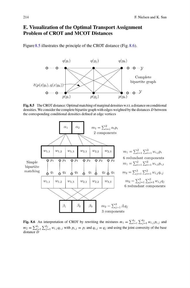
Figure 8.5 illustrates the principle of the CROT distance (Fig. 8.6).
Y
Y
p(y i )
p(y j )
p(y k )
q(y i )
q(y j )
q(y k )
δ(p(x|y i ), q(x|y k ))
Complete
bipartite graph
Fig. 8.5 The CROT distance: Optimal matching of marginal densities w.r.t. a distance on conditional
densities. We consider the complete bipartite graph with edges weighted by the distances D between
the corresponding conditional densities defined at edge vertices
α 1
α 2
β 1
β 2
β 3
w 1,1 w 1,2 w 1,3
w 2,1 w 2,2
w 2,3
m 1 =
2
i=1 α i p i
m 1 =
2
i=1
3
i=1 w i,j p i
Simple
bipartite
matching
m 2 =
3
j=1 β i q j
m 2 =
3
j=1
2
i=1 w i,j q j
2 components
6 redundant components
6 redundant components
3 components
m 2 =
3
j=1
2
i=1 w i,j q i,j
m 1 =
2
i=1
3
i=1 w i,j p i,j
p 1
p 1
p 1
p 2
p 2
p 2
q 1
q 2
q 3
q 1
w 1,1 w 1,2 w 1,3
w 2,1 w 2,2
w 3,3
q 2
q 3
Fig. 8.6 An interpretation of CROT by rewriting the mixtures m 1 =
k1
i=1
k2
j=1 w i, j p i, j and
m 2 =
k1
i=1
k2
j=1 w i, j q i, j with p i, j = p i and q i, j = q j and using the joint convexity of the base
distance D
F. Nielsen and K. Sun
E. Visualization of the Optimal Transport Assignment
Problem of CROT and MCOT Distances
Figure 8.5 illustrates the principle of the CROT distance (Fig. 8.6).
Y
Y
p(y i )
p(y j )
p(y k )
q(y i )
q(y j )
q(y k )
δ(p(x|y i ), q(x|y k ))
Complete
bipartite graph
Fig. 8.5 The CROT distance: Optimal matching of marginal densities w.r.t. a distance on conditional
densities. We consider the complete bipartite graph with edges weighted by the distances D between
the corresponding conditional densities defined at edge vertices
α 1
α 2
β 1
β 2
β 3
w 1,1 w 1,2 w 1,3
w 2,1 w 2,2
w 2,3
m 1 =
2
i=1 α i p i
m 1 =
2
i=1
3
i=1 w i,j p i
Simple
bipartite
matching
m 2 =
3
j=1 β i q j
m 2 =
3
j=1
2
i=1 w i,j q j
2 components
6 redundant components
6 redundant components
3 components
m 2 =
3
j=1
2
i=1 w i,j q i,j
m 1 =
2
i=1
3
i=1 w i,j p i,j
p 1
p 1
p 1
p 2
p 2
p 2
q 1
q 2
q 3
q 1
w 1,1 w 1,2 w 1,3
w 2,1 w 2,2
w 3,3
q 2
q 3
Fig. 8.6 An interpretation of CROT by rewriting the mixtures m 1 =
k1
i=1
k2
j=1 w i, j p i, j and
m 2 =
k1
i=1
k2
j=1 w i, j q i, j with p i, j = p i and q i, j = q j and using the joint convexity of the base
distance D