

8 Chain Rule Optimal Transport
213
10
1
10
2
10
3
0.0
0.5
1.0
√ JS 0.1
CEUB
CGQLB
CROT
MC
Cα
Sinkhorn
10
1
10
2
10
3
0.0
0.5
1.0
√ JS 0.5
CEUB
CGQLB
CROT
MC
Cα
Sinkhorn
10
1
10
2
10
3
0
1
2
√ JS 0.9
CEUB
CGQLB
CROT
MC
Cα
Sinkhorn
10
1
10
2
10
3
0.0
0.5
1.0
JS 0.1
CEUB
CGQLB
CROT
MC
Cα
Sinkhorn
10
1
10
2
10
3
0.0
0.5
1.0
JS 0.5
CEUB
CGQLB
CROT
MC
Cα
Sinkhorn
10
1
10
2
10
3
0
1
2
JS 0.9
CEUB
CGQLB
CROT
MC
Cα
Sinkhorn
10
1
10
2
10
3
0.0
0.5
1.0
√ JS 0.1
CEUB
CGQLB
CROT
MC
Cα
Sinkhorn
10
1
10
2
10
3
0.0
0.5
1.0
√ JS 0.5
CEUB
CGQLB
CROT
MC
Cα
Sinkhorn
10
1
10
2
10
3
0
1
2
√ JS 0.9
CEUB
CGQLB
CROT
MC
Cα
Sinkhorn
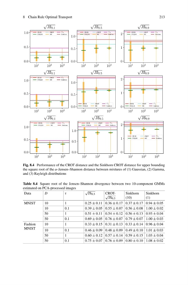
Fig. 8.4 Performance of the CROT distance and the Sinkhorn CROT distance for upper bounding
the square root of the α-Jensen–Shannon distance between mixtures of (1) Gaussian, (2) Gamma,
and (3) Rayleigh distributions
Table 8.4 Square root of the Jensen–Shannon divergence between two 10-component GMMs
estimated on PCA-processed images
Data
D
τ
√
JS 0.5
CROT- √
JS 0.5
Sinkhorn
(10)
Sinkhorn
(1)
MNIST
10
1
0.25 ± 0.11 0.36 ± 0.17 0.37 ± 0.17 0.94 ± 0.05
10
0.1
0.39 ± 0.05 0.55 ± 0.07 0.56 ± 0.08 1.00 ± 0.02
50
1
0.51 ± 0.11 0.54 ± 0.12 0.56 ± 0.13 0.93 ± 0.04
50
0.1
0.69 ± 0.05 0.76 ± 0.07 0.79 ± 0.07 1.00 ± 0.03
Fashion
MNIST
10
1
0.33 ± 0.15 0.31 ± 0.13 0.33 ± 0.14 0.96 ± 0.04
10
0.1
0.46 ± 0.09 0.48 ± 0.09 0.49 ± 0.10 1.01 ± 0.03
50
1
0.60 ± 0.12 0.57 ± 0.14 0.59 ± 0.15 1.03 ± 0.04
50
0.1
0.75 ± 0.07 0.76 ± 0.09 0.80 ± 0.10 1.08 ± 0.02
213
10
1
10
2
10
3
0.0
0.5
1.0
√ JS 0.1
CEUB
CGQLB
CROT
MC
Cα
Sinkhorn
10
1
10
2
10
3
0.0
0.5
1.0
√ JS 0.5
CEUB
CGQLB
CROT
MC
Cα
Sinkhorn
10
1
10
2
10
3
0
1
2
√ JS 0.9
CEUB
CGQLB
CROT
MC
Cα
Sinkhorn
10
1
10
2
10
3
0.0
0.5
1.0
JS 0.1
CEUB
CGQLB
CROT
MC
Cα
Sinkhorn
10
1
10
2
10
3
0.0
0.5
1.0
JS 0.5
CEUB
CGQLB
CROT
MC
Cα
Sinkhorn
10
1
10
2
10
3
0
1
2
JS 0.9
CEUB
CGQLB
CROT
MC
Cα
Sinkhorn
10
1
10
2
10
3
0.0
0.5
1.0
√ JS 0.1
CEUB
CGQLB
CROT
MC
Cα
Sinkhorn
10
1
10
2
10
3
0.0
0.5
1.0
√ JS 0.5
CEUB
CGQLB
CROT
MC
Cα
Sinkhorn
10
1
10
2
10
3
0
1
2
√ JS 0.9
CEUB
CGQLB
CROT
MC
Cα
Sinkhorn
Fig. 8.4 Performance of the CROT distance and the Sinkhorn CROT distance for upper bounding
the square root of the α-Jensen–Shannon distance between mixtures of (1) Gaussian, (2) Gamma,
and (3) Rayleigh distributions
Table 8.4 Square root of the Jensen–Shannon divergence between two 10-component GMMs
estimated on PCA-processed images
Data
D
τ
√
JS 0.5
CROT- √
JS 0.5
Sinkhorn
(10)
Sinkhorn
(1)
MNIST
10
1
0.25 ± 0.11 0.36 ± 0.17 0.37 ± 0.17 0.94 ± 0.05
10
0.1
0.39 ± 0.05 0.55 ± 0.07 0.56 ± 0.08 1.00 ± 0.02
50
1
0.51 ± 0.11 0.54 ± 0.12 0.56 ± 0.13 0.93 ± 0.04
50
0.1
0.69 ± 0.05 0.76 ± 0.07 0.79 ± 0.07 1.00 ± 0.03
Fashion
MNIST
10
1
0.33 ± 0.15 0.31 ± 0.13 0.33 ± 0.14 0.96 ± 0.04
10
0.1
0.46 ± 0.09 0.48 ± 0.09 0.49 ± 0.10 1.01 ± 0.03
50
1
0.60 ± 0.12 0.57 ± 0.14 0.59 ± 0.15 1.03 ± 0.04
50
0.1
0.75 ± 0.07 0.76 ± 0.09 0.80 ± 0.10 1.08 ± 0.02