

206
F. Nielsen and K. Sun
where λ > 0 is a regularization strength parameter (same as the Sinkhorn algorithm).
By a similar analysis [8], the optimal weights w
i j must satisfy
w
i j =
1
n
exp(−λKL( p i , q j ))
m
j=1 exp(−λKL( p i , q j ))
,
(8.15)
We therefore minimize
n
i=1
m
j=1 w
i j KL( p i , q j ) based on gradient descent on
mini-batches of n
samples. We set empirically the hyper-parameter m = 10 (number
of components), λ = 0.005 (Sinkhorn regularization parameter) and = 10
−6 (KDE
bandwidth). Fine tuning them can potentially yields better results. We use the training
dataset to learn the q distribution (GMM) and estimate the testing error based on its
distance with ˆ
p, a KDE w.r.t. the testing datasets.
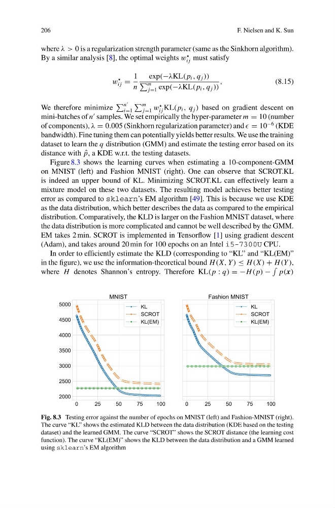
Figure 8.3 shows the learning curves when estimating a 10-component-GMM
on MNIST (left) and Fashion MNIST (right). One can observe that SCROT.KL
is indeed an upper bound of KL. Minimizing SCROT.KL can effectively learn a
mixture model on these two datasets. The resulting model achieves better testing
error as compared to sklearn’s EM algorithm [49]. This is because we use KDE
as the data distribution, which better describes the data as compared to the empirical
distribution. Comparatively, the KLD is larger on the Fashion MNIST dataset, where
the data distribution is more complicated and cannot be well described by the GMM.
EM takes 2 min. SCROT is implemented in Tensorflow [1] using gradient descent
(Adam), and takes around 20 min for 100 epochs on an Intel i5-7300U CPU.
In order to efficiently estimate the KLD (corresponding to “KL” and “KL(EM)”
in the figure), we use the information-theoretical bound H (X, Y ) ≤ H (X ) + H (Y ),
where H denotes Shannon’s entropy. Therefore KL( p : q) = −H ( p) −
p(x)
Fig. 8.3 Testing error against the number of epochs on MNIST (left) and Fashion-MNIST (right).
The curve “KL” shows the estimated KLD between the data distribution (KDE based on the testing
dataset) and the learned GMM. The curve “SCROT” shows the SCROT distance (the learning cost
function). The curve “KL(EM)” shows the KLD between the data distribution and a GMM learned
using sklearn’s EM algorithm
F. Nielsen and K. Sun
where λ > 0 is a regularization strength parameter (same as the Sinkhorn algorithm).
By a similar analysis [8], the optimal weights w
i j must satisfy
w
i j =
1
n
exp(−λKL( p i , q j ))
m
j=1 exp(−λKL( p i , q j ))
,
(8.15)
We therefore minimize
n
i=1
m
j=1 w
i j KL( p i , q j ) based on gradient descent on
mini-batches of n
samples. We set empirically the hyper-parameter m = 10 (number
of components), λ = 0.005 (Sinkhorn regularization parameter) and = 10
−6 (KDE
bandwidth). Fine tuning them can potentially yields better results. We use the training
dataset to learn the q distribution (GMM) and estimate the testing error based on its
distance with ˆ
p, a KDE w.r.t. the testing datasets.
Figure 8.3 shows the learning curves when estimating a 10-component-GMM
on MNIST (left) and Fashion MNIST (right). One can observe that SCROT.KL
is indeed an upper bound of KL. Minimizing SCROT.KL can effectively learn a
mixture model on these two datasets. The resulting model achieves better testing
error as compared to sklearn’s EM algorithm [49]. This is because we use KDE
as the data distribution, which better describes the data as compared to the empirical
distribution. Comparatively, the KLD is larger on the Fashion MNIST dataset, where
the data distribution is more complicated and cannot be well described by the GMM.
EM takes 2 min. SCROT is implemented in Tensorflow [1] using gradient descent
(Adam), and takes around 20 min for 100 epochs on an Intel i5-7300U CPU.
In order to efficiently estimate the KLD (corresponding to “KL” and “KL(EM)”
in the figure), we use the information-theoretical bound H (X, Y ) ≤ H (X ) + H (Y ),
where H denotes Shannon’s entropy. Therefore KL( p : q) = −H ( p) −
p(x)
Fig. 8.3 Testing error against the number of epochs on MNIST (left) and Fashion-MNIST (right).
The curve “KL” shows the estimated KLD between the data distribution (KDE based on the testing
dataset) and the learned GMM. The curve “SCROT” shows the SCROT distance (the learning cost
function). The curve “KL(EM)” shows the KLD between the data distribution and a GMM learned
using sklearn’s EM algorithm