

204
F. Nielsen and K. Sun
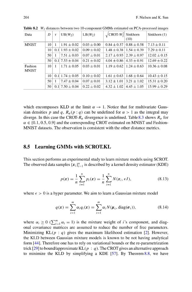
Table 8.2 W 2 distances between two 10-component GMMs estimated on PCA-processed images
Data
D τ UB(W 2 )
LB(W 2 )
CROT-W 2
2 Sinkhorn
(10)
Sinkhorn (1)
MNIST
10 1 1.91 ± 0.02 0.03 ± 0.00 0.84 ± 0.57 0.88 ± 0.58 7.13 ± 0.11
10 0.1 1.93 ± 0.02 0.09 ± 0.02 1.48 ± 0.38 1.54 ± 0.39 7.29 ± 0.11
50 1 7.51 ± 0.03 0.07 ± 0.01 2.17 ± 0.93 2.39 ± 0.97 12.02 ± 0.15
50 0.1 7.53 ± 0.04 0.21 ± 0.02 4.04 ± 0.86 4.33 ± 0.91 12.69 ± 0.22
Fashion
MNIST
10 1 1.71 ± 0.05 0.03 ± 0.01 1.19 ± 0.62 1.24 ± 0.63 10.36 ± 0.08
10 0.1 1.74 ± 0.05 0.10 ± 0.02 1.61 ± 0.63 1.68 ± 0.64 10.43 ± 0.15
50 1 7.47 ± 0.04 0.07 ± 0.01 3.12 ± 1.01 3.21 ± 1.02 15.31 ± 0.20
50 0.1 7.50 ± 0.04 0.22 ± 0.02 4.32 ± 1.02 4.45 ± 1.05 15.99 ± 0.29
which encompasses KLD at the limit α → 1. Notice that for multivariate Gaussian densities p and q, R α ( p : q) can be undefined for α > 1 as the integral may
diverge. In this case the CROT-R α divergence is undefined. Table 8.3 shows R α for
α ∈ {0.1, 0.5, 0.9} and the corresponding CROT estimated on MNIST and FashionMNIST datasets. The observation is consistent with the other distance metrics.
8.5 Learning GMMs with SCROT.KL
This section performs an experimental study to learn mixture models using SCROT.
The observed data samples {x i }
n
i=1 is described by a kernel density estimator (KDE)
p(x) =
1
n
n
i=1
p i (x) =
1
n
n
i=1
N (x i , , I ),
(8.13)
where > 0 is a hyper parameter. We aim to learn a Gaussian mixture model
q(x) =
m
i=1
α i q i (x) =
m
i=1
α i N (μ i , diag(σ i )),
(8.14)
where α i ≥ 0 (
m
i=1 α i = 1) is the mixture weight of i’s component, and diagonal covariance matrices are assumed to reduce the number of free parameters.
Minimizing KL( p : q) gives the maximum likelihood estimation [2]. However,
the KLD between Gaussian mixture models is known to be not having analytical
form [44]. Therefore one has to rely on variational bounds or the re-parametrization
trick [29] to bound/approximate KL( p : q). The CROT gives an alternative approach
to minimize the KLD by simplifying a KDE [57]. By Theorem 8.8, we have
F. Nielsen and K. Sun
Table 8.2 W 2 distances between two 10-component GMMs estimated on PCA-processed images
Data
D τ UB(W 2 )
LB(W 2 )
CROT-W 2
2 Sinkhorn
(10)
Sinkhorn (1)
MNIST
10 1 1.91 ± 0.02 0.03 ± 0.00 0.84 ± 0.57 0.88 ± 0.58 7.13 ± 0.11
10 0.1 1.93 ± 0.02 0.09 ± 0.02 1.48 ± 0.38 1.54 ± 0.39 7.29 ± 0.11
50 1 7.51 ± 0.03 0.07 ± 0.01 2.17 ± 0.93 2.39 ± 0.97 12.02 ± 0.15
50 0.1 7.53 ± 0.04 0.21 ± 0.02 4.04 ± 0.86 4.33 ± 0.91 12.69 ± 0.22
Fashion
MNIST
10 1 1.71 ± 0.05 0.03 ± 0.01 1.19 ± 0.62 1.24 ± 0.63 10.36 ± 0.08
10 0.1 1.74 ± 0.05 0.10 ± 0.02 1.61 ± 0.63 1.68 ± 0.64 10.43 ± 0.15
50 1 7.47 ± 0.04 0.07 ± 0.01 3.12 ± 1.01 3.21 ± 1.02 15.31 ± 0.20
50 0.1 7.50 ± 0.04 0.22 ± 0.02 4.32 ± 1.02 4.45 ± 1.05 15.99 ± 0.29
which encompasses KLD at the limit α → 1. Notice that for multivariate Gaussian densities p and q, R α ( p : q) can be undefined for α > 1 as the integral may
diverge. In this case the CROT-R α divergence is undefined. Table 8.3 shows R α for
α ∈ {0.1, 0.5, 0.9} and the corresponding CROT estimated on MNIST and FashionMNIST datasets. The observation is consistent with the other distance metrics.
8.5 Learning GMMs with SCROT.KL
This section performs an experimental study to learn mixture models using SCROT.
The observed data samples {x i }
n
i=1 is described by a kernel density estimator (KDE)
p(x) =
1
n
n
i=1
p i (x) =
1
n
n
i=1
N (x i , , I ),
(8.13)
where > 0 is a hyper parameter. We aim to learn a Gaussian mixture model
q(x) =
m
i=1
α i q i (x) =
m
i=1
α i N (μ i , diag(σ i )),
(8.14)
where α i ≥ 0 (
m
i=1 α i = 1) is the mixture weight of i’s component, and diagonal covariance matrices are assumed to reduce the number of free parameters.
Minimizing KL( p : q) gives the maximum likelihood estimation [2]. However,
the KLD between Gaussian mixture models is known to be not having analytical
form [44]. Therefore one has to rely on variational bounds or the re-parametrization
trick [29] to bound/approximate KL( p : q). The CROT gives an alternative approach
to minimize the KLD by simplifying a KDE [57]. By Theorem 8.8, we have