

202
F. Nielsen and K. Sun
Figure 8.3(1) shows the 10 × 10 TV distance between mm1’s components and
mm2’s components red means large distance, blue means a small distance Fig. 8.3
(Table 8.1).
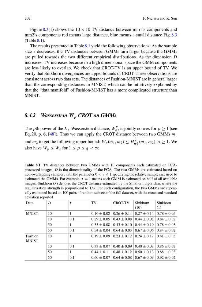
The results presented in Table 8.1 yield the following observations: As the sample
size τ decreases, the TV distances between GMMs turn larger because the GMMs
are pulled towards the two different empirical distributions. As the dimension D
increases, TV increases because in a high dimensional space the GMM components
are less likely to overlap. We check that CROT-TV is an upper bound of TV. We
verify that Sinkhorn divergences are upper bounds of CROT. These observations are
consistent across two data sets. The distances of Fashion-MNIST are in general larger
than the corresponding distances in MNIST, which can be intuitively explained by
that the “data manifold” of Fashion-MNIST has a more complicated structure than
MNIST.
8.4.2 Wasserstein W p CROT on GMMs
The pth power of the L p -Wasserstein distance, W
p
p , is jointly convex for p ≥ 1 (see
Eq. 20, p. 6, [48]). Thus we can apply the CROT distance between two GMMs m 1
and m 2 to get the following upper bound: W p (m 1 , m 2 ) ≤ H
1
p
W
p
p
(m 1 , m 2 ), α ≥ 1. We
also have W p ≤ W q for 1 ≤ p ≤ q < ∞.
Table 8.1 TV distances between two GMMs with 10 components each estimated on PCAprocessed images. D is the dimensionality of the PCA. The two GMMs are estimated based on
non-overlapping samples, with the parameter 0 < τ ≤ 1 specifying the relative sample size used to
estimated the GMMs. For example, τ = 1 means each GMM is estimated on half of all available
images. Sinkhorn (λ) denotes the CROT distance estimated by the Sinkhorn algorithm, where the
regularization strength is proportional to 1/λ. For each configuration, the two GMMs are repeatedly estimated based on 100 pairs of random subsets of the full dataset, with the mean and standard
deviation reported
Data
D
τ
TV
CROT-TV Sinkhorn
(10)
Sinkhorn
(1)
MNIST
10
1
0.16 ± 0.08 0.26 ± 0.14 0.27 ± 0.14 0.78 ± 0.05
10
0.1
0.29 ± 0.05 0.43 ± 0.08 0.44 ± 0.08 0.84 ± 0.02
50
1
0.35 ± 0.08 0.43 ± 0.10 0.44 ± 0.10 0.78 ± 0.03
50
0.1
0.54 ± 0.04 0.64 ± 0.05 0.67 ± 0.06 0.84 ± 0.02
Fashion
MNIST
10
1
0.19 ± 0.09 0.23 ± 0.12 0.24 ± 0.12 0.81 ± 0.03
10
0.1
0.33 ± 0.07 0.40 ± 0.09 0.40 ± 0.09 0.86 ± 0.02
50
1
0.44 ± 0.11 0.48 ± 0.12 0.50 ± 0.13 0.88 ± 0.03
50
0.1
0.60 ± 0.07 0.64 ± 0.08 0.67 ± 0.09 0.92 ± 0.02
F. Nielsen and K. Sun
Figure 8.3(1) shows the 10 × 10 TV distance between mm1’s components and
mm2’s components red means large distance, blue means a small distance Fig. 8.3
(Table 8.1).
The results presented in Table 8.1 yield the following observations: As the sample
size τ decreases, the TV distances between GMMs turn larger because the GMMs
are pulled towards the two different empirical distributions. As the dimension D
increases, TV increases because in a high dimensional space the GMM components
are less likely to overlap. We check that CROT-TV is an upper bound of TV. We
verify that Sinkhorn divergences are upper bounds of CROT. These observations are
consistent across two data sets. The distances of Fashion-MNIST are in general larger
than the corresponding distances in MNIST, which can be intuitively explained by
that the “data manifold” of Fashion-MNIST has a more complicated structure than
MNIST.
8.4.2 Wasserstein W p CROT on GMMs
The pth power of the L p -Wasserstein distance, W
p
p , is jointly convex for p ≥ 1 (see
Eq. 20, p. 6, [48]). Thus we can apply the CROT distance between two GMMs m 1
and m 2 to get the following upper bound: W p (m 1 , m 2 ) ≤ H
1
p
W
p
p
(m 1 , m 2 ), α ≥ 1. We
also have W p ≤ W q for 1 ≤ p ≤ q < ∞.
Table 8.1 TV distances between two GMMs with 10 components each estimated on PCAprocessed images. D is the dimensionality of the PCA. The two GMMs are estimated based on
non-overlapping samples, with the parameter 0 < τ ≤ 1 specifying the relative sample size used to
estimated the GMMs. For example, τ = 1 means each GMM is estimated on half of all available
images. Sinkhorn (λ) denotes the CROT distance estimated by the Sinkhorn algorithm, where the
regularization strength is proportional to 1/λ. For each configuration, the two GMMs are repeatedly estimated based on 100 pairs of random subsets of the full dataset, with the mean and standard
deviation reported
Data
D
τ
TV
CROT-TV Sinkhorn
(10)
Sinkhorn
(1)
MNIST
10
1
0.16 ± 0.08 0.26 ± 0.14 0.27 ± 0.14 0.78 ± 0.05
10
0.1
0.29 ± 0.05 0.43 ± 0.08 0.44 ± 0.08 0.84 ± 0.02
50
1
0.35 ± 0.08 0.43 ± 0.10 0.44 ± 0.10 0.78 ± 0.03
50
0.1
0.54 ± 0.04 0.64 ± 0.05 0.67 ± 0.06 0.84 ± 0.02
Fashion
MNIST
10
1
0.19 ± 0.09 0.23 ± 0.12 0.24 ± 0.12 0.81 ± 0.03
10
0.1
0.33 ± 0.07 0.40 ± 0.09 0.40 ± 0.09 0.86 ± 0.02
50
1
0.44 ± 0.11 0.48 ± 0.12 0.50 ± 0.13 0.88 ± 0.03
50
0.1
0.60 ± 0.07 0.64 ± 0.08 0.67 ± 0.09 0.92 ± 0.02