

8 Chain Rule Optimal Transport
201
0
10
20
30
0.0
0.2
0.4
RMM 1
0
100
200
300
0.00
0.01
0.02
0.03
RMM 2
10
1
10
2
10
3
0.0
0.5
1.0
TV
CELB
CEUB
CGQLB
CROT
MC
Sinkhorn
−2.5
0.0
2.5
0.0
0.1
0.2
GMM 3
−5.0
−2.5
0.0
2.5
0.0
0.2
0.4
0.6
GMM 4
10
1
10
2
10
3
0.0
0.5
1.0
TV
CELB
CEUB
CGQLB
CROT
MC
Sinkhorn
0
10
0.0
0.1
0.2
GaMM 1
0
20
40
0.00
0.01
0.02
GaMM 2
10
1
10
2
10
3
0.0
0.5
1.0
TV
CELB
CEUB
CGQLB
CROT
MC
Sinkhorn
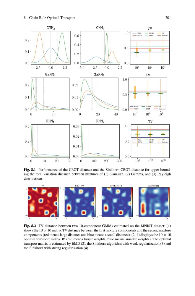
Fig. 8.1 Performance of the CROT distance and the Sinkhorn CROT distance for upper bounding the total variation distance between mixtures of (1) Gaussian, (2) Gamma, and (3) Rayleigh
distributions
Fig. 8.2 TV distance between two 10-component GMMs estimated on the MNIST dataset: (1)
shows the 10 × 10 matrix TV distance between the first mixture components and the second mixture
components (red means large distance and blue means a small distance). (2–4) displays the 10 × 10
optimal transport matrix W (red means larger weights, blue means smaller weights). The optimal
transport matrix is estimated by EMD (2), the Sinkhorn algorithm with weak regularization (3) and
the Sinkhorn with strong regularization (4)
201
0
10
20
30
0.0
0.2
0.4
RMM 1
0
100
200
300
0.00
0.01
0.02
0.03
RMM 2
10
1
10
2
10
3
0.0
0.5
1.0
TV
CELB
CEUB
CGQLB
CROT
MC
Sinkhorn
−2.5
0.0
2.5
0.0
0.1
0.2
GMM 3
−5.0
−2.5
0.0
2.5
0.0
0.2
0.4
0.6
GMM 4
10
1
10
2
10
3
0.0
0.5
1.0
TV
CELB
CEUB
CGQLB
CROT
MC
Sinkhorn
0
10
0.0
0.1
0.2
GaMM 1
0
20
40
0.00
0.01
0.02
GaMM 2
10
1
10
2
10
3
0.0
0.5
1.0
TV
CELB
CEUB
CGQLB
CROT
MC
Sinkhorn
Fig. 8.1 Performance of the CROT distance and the Sinkhorn CROT distance for upper bounding the total variation distance between mixtures of (1) Gaussian, (2) Gamma, and (3) Rayleigh
distributions
Fig. 8.2 TV distance between two 10-component GMMs estimated on the MNIST dataset: (1)
shows the 10 × 10 matrix TV distance between the first mixture components and the second mixture
components (red means large distance and blue means a small distance). (2–4) displays the 10 × 10
optimal transport matrix W (red means larger weights, blue means smaller weights). The optimal
transport matrix is estimated by EMD (2), the Sinkhorn algorithm with weak regularization (3) and
the Sinkhorn with strong regularization (4)