

8 Chain Rule Optimal Transport
199
as mixtures of k = k 1 × k 2 (redundant) components { p i, j (x) = p i (x)} and {q i, j (x) =
q j (x)}, and apply the upper bound of Eq. 8.9 for the “best split” of matching mixture
components
k 2
j=1 w i, j p i (x) ↔
k 1
j=1 w
j,i q i (x):
KL(m 1 : m 2 ) ≤ O(m 1 : m 2 ) ≤
k 1
i=1
k 2
j=1
w i, j log
w i, j
w
j,i
+ H KL (m 1 , m 2 ),
where
O(m 1 : m 2 ) = min
w∈U (α,β)
k 1
i=1
k 2
j=1
w i, j log
w i, j
w
j,i
+
k 1
i=1
k 2
j=1
w i j KL( p i : q j ).
(8.11)
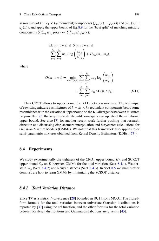
Thus CROT allows to upper bound the KLD between mixtures. The technique
of rewriting mixtures as mixtures of k = k 1 × k 2 redundant components bears some
resemblance with the variational upper bound on the KL divergence between mixtures
proposed by [25] that requires to iterate until convergence an update of the variational
upper bound. See also [7] for another recent work further pushing that research
direction and discussing displacement interpolation and barycenter calculations for
Gaussian Mixture Models (GMMs). We note that this framework also applies to or
semi-parametric mixtures obtained from Kernel Density Estimators (KDEs; [57]).
8.4 Experiments
We study experimentally the tightness of the CROT upper bound H D and SCROT
upper bound S D on D between GMMs for the total variation (Sect. 8.4.1), Wasserstein W p (Sect. 8.4.2) and Rényi distances (Sect. 8.4.3). In Sect. 8.5 we shall further
demonstrate how to learn GMMs by minimizing the SCROT distance.
8.4.1 Total Variation Distance
Since TV is a metric f -divergence [28] bounded in [0, 1], so is MCOT. The closedform formula for the total variation between univariate Gaussian distributions is
reported by [37] using the erf function, and the other formula for the total variation
between Rayleigh distributions and Gamma distributions are given in [45].
199
as mixtures of k = k 1 × k 2 (redundant) components { p i, j (x) = p i (x)} and {q i, j (x) =
q j (x)}, and apply the upper bound of Eq. 8.9 for the “best split” of matching mixture
components
k 2
j=1 w i, j p i (x) ↔
k 1
j=1 w
j,i q i (x):
KL(m 1 : m 2 ) ≤ O(m 1 : m 2 ) ≤
k 1
i=1
k 2
j=1
w i, j log
w i, j
w
j,i
+ H KL (m 1 , m 2 ),
where
O(m 1 : m 2 ) = min
w∈U (α,β)
k 1
i=1
k 2
j=1
w i, j log
w i, j
w
j,i
+
k 1
i=1
k 2
j=1
w i j KL( p i : q j ).
(8.11)
Thus CROT allows to upper bound the KLD between mixtures. The technique
of rewriting mixtures as mixtures of k = k 1 × k 2 redundant components bears some
resemblance with the variational upper bound on the KL divergence between mixtures
proposed by [25] that requires to iterate until convergence an update of the variational
upper bound. See also [7] for another recent work further pushing that research
direction and discussing displacement interpolation and barycenter calculations for
Gaussian Mixture Models (GMMs). We note that this framework also applies to or
semi-parametric mixtures obtained from Kernel Density Estimators (KDEs; [57]).
8.4 Experiments
We study experimentally the tightness of the CROT upper bound H D and SCROT
upper bound S D on D between GMMs for the total variation (Sect. 8.4.1), Wasserstein W p (Sect. 8.4.2) and Rényi distances (Sect. 8.4.3). In Sect. 8.5 we shall further
demonstrate how to learn GMMs by minimizing the SCROT distance.
8.4.1 Total Variation Distance
Since TV is a metric f -divergence [28] bounded in [0, 1], so is MCOT. The closedform formula for the total variation between univariate Gaussian distributions is
reported by [37] using the erf function, and the other formula for the total variation
between Rayleigh distributions and Gamma distributions are given in [45].