

180
F. Nielsen
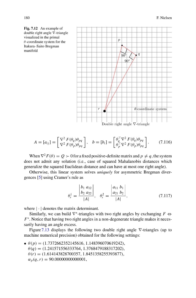
Fig. 7.12 An example of
double right angle ∇-triangle
visualized in the primal
θ-coordinate system for the
Itakura–Saito Bregman
manifold
r
p
q
θ-coordinate system
90
o
90
o
Double right angle -triangle
A = [a i j ] =
∇
2 F(θ q )θ pq
∇
2 F(θ p )θ pq
, b = [b i ] =
θ
q ∇
2 F(θ q )θ pq
θ
p ∇
2 F(θ p )θ pq
.
(7.116)
When ∇
2 F(θ ) = Q 0 for a fixed positive-definite matrix and p = q, the system
does not admit any solution (i.e., case of squared Mahalanobis distances which
generalize the squared Euclidean distance and can have at most one right angle).
Otherwise, this linear system solves uniquely for asymmetric Bregman divergences [5] using Cramer’s rule as
θ
1
r =
b 1 a 12
b 2 a 22
|A|
, θ
2
r =
a 11 b 1
a 21 b 2
|A|
,
(7.117)
where | · | denotes the matrix determinant.
Similarly, we can build ∇
∗ -triangles with two right angles by exchanging F ⇔
F
∗ . Notice that having two right angles in a non-degenerate triangle makes it necessarily having an angle excess.
Figure 7.13 displays the following two double right angle ∇-triangles (up to
machine numerical precision) obtained for the following settings:
• θ( p) = (1.7372662352145616, 1.148396070619242),
θ(q) = (1.241571556333764, 1.3768479188317202),
θ(r ) = (1.614143828700357, 1.8451358255393877),
α p (q, r ) = 90.00000000000001,
F. Nielsen
Fig. 7.12 An example of
double right angle ∇-triangle
visualized in the primal
θ-coordinate system for the
Itakura–Saito Bregman
manifold
r
p
q
θ-coordinate system
90
o
90
o
Double right angle -triangle
A = [a i j ] =
∇
2 F(θ q )θ pq
∇
2 F(θ p )θ pq
, b = [b i ] =
θ
q ∇
2 F(θ q )θ pq
θ
p ∇
2 F(θ p )θ pq
.
(7.116)
When ∇
2 F(θ ) = Q 0 for a fixed positive-definite matrix and p = q, the system
does not admit any solution (i.e., case of squared Mahalanobis distances which
generalize the squared Euclidean distance and can have at most one right angle).
Otherwise, this linear system solves uniquely for asymmetric Bregman divergences [5] using Cramer’s rule as
θ
1
r =
b 1 a 12
b 2 a 22
|A|
, θ
2
r =
a 11 b 1
a 21 b 2
|A|
,
(7.117)
where | · | denotes the matrix determinant.
Similarly, we can build ∇
∗ -triangles with two right angles by exchanging F ⇔
F
∗ . Notice that having two right angles in a non-degenerate triangle makes it necessarily having an angle excess.
Figure 7.13 displays the following two double right angle ∇-triangles (up to
machine numerical precision) obtained for the following settings:
• θ( p) = (1.7372662352145616, 1.148396070619242),
θ(q) = (1.241571556333764, 1.3768479188317202),
θ(r ) = (1.614143828700357, 1.8451358255393877),
α p (q, r ) = 90.00000000000001,