

176
F. Nielsen
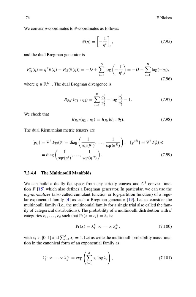
We convex η-coordinates to θ -coordinates as follows:
θ(η) =
−
1
η i
i
,
(7.95)
and the dual Bregman generator is
F
∗
IS (η) = η
θ(η) − F IS (θ (η)) = −D +
D
i=1
log
−
1
η i
= −D −
D
i=1
log(−η i ),
(7.96)
where η ∈ R
D
−− . The dual Bregman divergence is
B F IS
∗ (η 1 : η 2 ) =
D
i=1
η
i
1
η
i
2
− log
η
i
1
η
i
2
− 1.
(7.97)
We check that
B F IS
∗ (η 2 : η 1 ) = B F IS (θ 1 : θ 2 ).
(7.98)
The dual Riemannian metric tensors are
[g i j ] = ∇
2 F IS (θ ) = diag
1
sqr(θ 1 )
, . . . ,
1
sqr(θ D )
, [g
∗i j ] = ∇
2 F
∗
IS (η)
= diag
1
sqr(η 1 )
, . . . ,
1
sqr(η D )
.
(7.99)
7.2.4.4 The Multinoulli Manifolds
We can build a dually flat space from any strictly convex and C
3 convex function F [15] which also defines a Bregman generator. In particular, we can use the
log-normalizer (also called cumulant function or log-partition function) of a regular exponential family [4] as such a Bregman generator [19]. Let us consider the
multinoulli family (i.e., the multinomial family for a single trial also called the family of categorical distributions). The probability of a multinoulli distribution with d
categories c 1 , . . . , c d such that Pr(x = c i ) = λ i is:
Pr(x) = λ
x 1
1 × · · · × λ
x d
d ,
(7.100)
with x i ∈ {0, 1} and
d
i=1 x i = 1. Let us write the multinoulli probability mass function in the canonical form of an exponential family as
λ
x 1
1 × · · · × λ
x d
d = exp
d
i=1
x i log λ i
,
(7.101)
F. Nielsen
We convex η-coordinates to θ -coordinates as follows:
θ(η) =
−
1
η i
i
,
(7.95)
and the dual Bregman generator is
F
∗
IS (η) = η
θ(η) − F IS (θ (η)) = −D +
D
i=1
log
−
1
η i
= −D −
D
i=1
log(−η i ),
(7.96)
where η ∈ R
D
−− . The dual Bregman divergence is
B F IS
∗ (η 1 : η 2 ) =
D
i=1
η
i
1
η
i
2
− log
η
i
1
η
i
2
− 1.
(7.97)
We check that
B F IS
∗ (η 2 : η 1 ) = B F IS (θ 1 : θ 2 ).
(7.98)
The dual Riemannian metric tensors are
[g i j ] = ∇
2 F IS (θ ) = diag
1
sqr(θ 1 )
, . . . ,
1
sqr(θ D )
, [g
∗i j ] = ∇
2 F
∗
IS (η)
= diag
1
sqr(η 1 )
, . . . ,
1
sqr(η D )
.
(7.99)
7.2.4.4 The Multinoulli Manifolds
We can build a dually flat space from any strictly convex and C
3 convex function F [15] which also defines a Bregman generator. In particular, we can use the
log-normalizer (also called cumulant function or log-partition function) of a regular exponential family [4] as such a Bregman generator [19]. Let us consider the
multinoulli family (i.e., the multinomial family for a single trial also called the family of categorical distributions). The probability of a multinoulli distribution with d
categories c 1 , . . . , c d such that Pr(x = c i ) = λ i is:
Pr(x) = λ
x 1
1 × · · · × λ
x d
d ,
(7.100)
with x i ∈ {0, 1} and
d
i=1 x i = 1. Let us write the multinoulli probability mass function in the canonical form of an exponential family as
λ
x 1
1 × · · · × λ
x d
d = exp
d
i=1
x i log λ i
,
(7.101)