

11 Structure and Electrical/Dielectric Properties of Ion-Conductive Polymer. . .
187
a)
b)
10
1 10
2 10
3 10
4 10
5 10
6 10
7 10
8
10
0
10
1
10
2
10
3
10
4
10
5
10
6
10
7
10
8
Z'', Ohm
Z', Ohm
40
60
80
100
140
200
20
<0
0
5
10
15
20
0
1
2
3
4
5
6
Z" 10
●
-5
, Ohm
Z' ● 10
-5 , Ohm
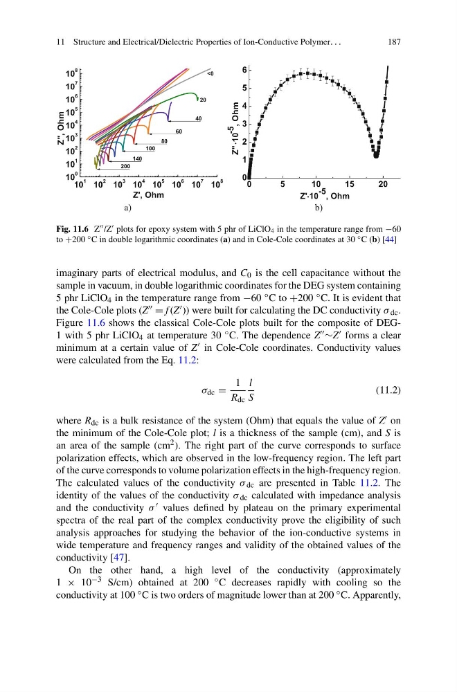
Fig. 11.6 Z /Z plots for epoxy system with 5 phr of LiClO 4 in the temperature range from −60
to +200 ◦ C in double logarithmic coordinates (a) and in Cole-Cole coordinates at 30 ◦ C (b) [44]
imaginary parts of electrical modulus, and C 0 is the cell capacitance without the
sample in vacuum, in double logarithmic coordinates for the DEG system containing
5 phr LiClO 4 in the temperature range from −60 ◦ C to +200 ◦ C. It is evident that
the Cole-Cole plots (Z = f (Z )) were built for calculating the DC conductivity σ dc .
Figure 11.6 shows the classical Cole-Cole plots built for the composite of DEG1 with 5 phr LiClO 4 at temperature 30 ◦ C. The dependence Z ∼Z forms a clear
minimum at a certain value of Z in Cole-Cole coordinates. Conductivity values
were calculated from the Eq. 11.2:
σ dc =
1
R dc
l
S
(11.2)
where R dc is a bulk resistance of the system (Ohm) that equals the value of Z on
the minimum of the Cole-Cole plot; l is a thickness of the sample (cm), and S is
an area of the sample (cm 2 ). The right part of the curve corresponds to surface
polarization effects, which are observed in the low-frequency region. The left part
of the curve corresponds to volume polarization effects in the high-frequency region.
The calculated values of the conductivity σ dc are presented in Table 11.2. The
identity of the values of the conductivity σ dc calculated with impedance analysis
and the conductivity σ values defined by plateau on the primary experimental
spectra of the real part of the complex conductivity prove the eligibility of such
analysis approaches for studying the behavior of the ion-conductive systems in
wide temperature and frequency ranges and validity of the obtained values of the
conductivity [47].
On the other hand, a high level of the conductivity (approximately
1 × 10 −3 S/cm) obtained at 200 ◦ C decreases rapidly with cooling so the
conductivity at 100 ◦ C is two orders of magnitude lower than at 200 ◦ C. Apparently,
187
a)
b)
10
1 10
2 10
3 10
4 10
5 10
6 10
7 10
8
10
0
10
1
10
2
10
3
10
4
10
5
10
6
10
7
10
8
Z'', Ohm
Z', Ohm
40
60
80
100
140
200
20
<0
0
5
10
15
20
0
1
2
3
4
5
6
Z" 10
●
-5
, Ohm
Z' ● 10
-5 , Ohm
Fig. 11.6 Z /Z plots for epoxy system with 5 phr of LiClO 4 in the temperature range from −60
to +200 ◦ C in double logarithmic coordinates (a) and in Cole-Cole coordinates at 30 ◦ C (b) [44]
imaginary parts of electrical modulus, and C 0 is the cell capacitance without the
sample in vacuum, in double logarithmic coordinates for the DEG system containing
5 phr LiClO 4 in the temperature range from −60 ◦ C to +200 ◦ C. It is evident that
the Cole-Cole plots (Z = f (Z )) were built for calculating the DC conductivity σ dc .
Figure 11.6 shows the classical Cole-Cole plots built for the composite of DEG1 with 5 phr LiClO 4 at temperature 30 ◦ C. The dependence Z ∼Z forms a clear
minimum at a certain value of Z in Cole-Cole coordinates. Conductivity values
were calculated from the Eq. 11.2:
σ dc =
1
R dc
l
S
(11.2)
where R dc is a bulk resistance of the system (Ohm) that equals the value of Z on
the minimum of the Cole-Cole plot; l is a thickness of the sample (cm), and S is
an area of the sample (cm 2 ). The right part of the curve corresponds to surface
polarization effects, which are observed in the low-frequency region. The left part
of the curve corresponds to volume polarization effects in the high-frequency region.
The calculated values of the conductivity σ dc are presented in Table 11.2. The
identity of the values of the conductivity σ dc calculated with impedance analysis
and the conductivity σ values defined by plateau on the primary experimental
spectra of the real part of the complex conductivity prove the eligibility of such
analysis approaches for studying the behavior of the ion-conductive systems in
wide temperature and frequency ranges and validity of the obtained values of the
conductivity [47].
On the other hand, a high level of the conductivity (approximately
1 × 10 −3 S/cm) obtained at 200 ◦ C decreases rapidly with cooling so the
conductivity at 100 ◦ C is two orders of magnitude lower than at 200 ◦ C. Apparently,