

14
S. A. Majid and S. Tripathi
volume. Further, the surface changes and the bed deviations are incorporated into the
flow domain using the interface tracking method (ITM) to increase computational
efficiency [2]. The bed deviations are calculated explicitly after the flow field has
been calculated for each time step. The advection terms are discretised using TVDMUSCL scheme (TVD: Taylor–Green vortex flow; MUSCL: monotone upstreamcentred scheme for conservation laws) which is a third-order accurate discretisation
scheme. The coefficient for Courant–Friedrichs–Lewy (CFL ) condition to determine the time step between two successive computations is set to 0.2. Six problems
of pressure scouring are simulated, and the details are given in Table 1.
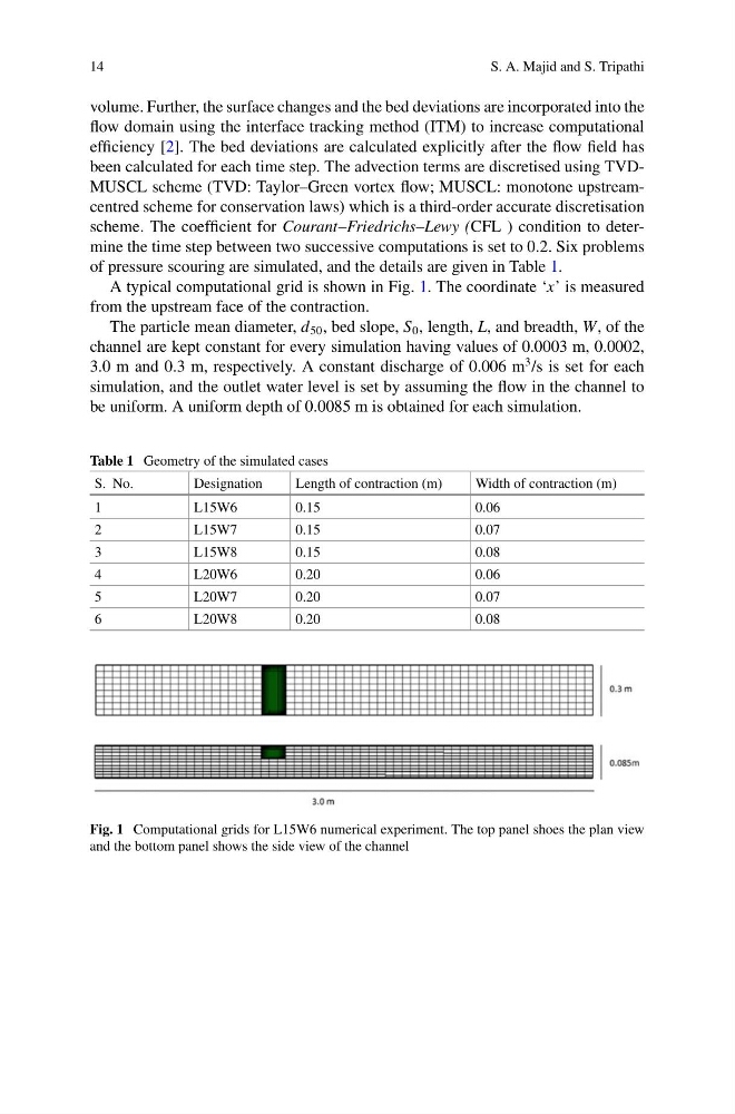
A typical computational grid is shown in Fig. 1. The coordinate ‘x’ is measured
from the upstream face of the contraction.
The particle mean diameter, d 50 , bed slope, S 0 , length, L, and breadth, W, of the
channel are kept constant for every simulation having values of 0.0003 m, 0.0002,
3.0 m and 0.3 m, respectively. A constant discharge of 0.006 m
3 /s is set for each
simulation, and the outlet water level is set by assuming the flow in the channel to
be uniform. A uniform depth of 0.0085 m is obtained for each simulation.
Table 1 Geometry of the simulated cases
S. No.
Designation
Length of contraction (m)
Width of contraction (m)
1
L15W6
0.15
0.06
2
L15W7
0.15
0.07
3
L15W8
0.15
0.08
4
L20W6
0.20
0.06
5
L20W7
0.20
0.07
6
L20W8
0.20
0.08
Fig. 1 Computational grids for L15W6 numerical experiment. The top panel shoes the plan view
and the bottom panel shows the side view of the channel
S. A. Majid and S. Tripathi
volume. Further, the surface changes and the bed deviations are incorporated into the
flow domain using the interface tracking method (ITM) to increase computational
efficiency [2]. The bed deviations are calculated explicitly after the flow field has
been calculated for each time step. The advection terms are discretised using TVDMUSCL scheme (TVD: Taylor–Green vortex flow; MUSCL: monotone upstreamcentred scheme for conservation laws) which is a third-order accurate discretisation
scheme. The coefficient for Courant–Friedrichs–Lewy (CFL ) condition to determine the time step between two successive computations is set to 0.2. Six problems
of pressure scouring are simulated, and the details are given in Table 1.
A typical computational grid is shown in Fig. 1. The coordinate ‘x’ is measured
from the upstream face of the contraction.
The particle mean diameter, d 50 , bed slope, S 0 , length, L, and breadth, W, of the
channel are kept constant for every simulation having values of 0.0003 m, 0.0002,
3.0 m and 0.3 m, respectively. A constant discharge of 0.006 m
3 /s is set for each
simulation, and the outlet water level is set by assuming the flow in the channel to
be uniform. A uniform depth of 0.0085 m is obtained for each simulation.
Table 1 Geometry of the simulated cases
S. No.
Designation
Length of contraction (m)
Width of contraction (m)
1
L15W6
0.15
0.06
2
L15W7
0.15
0.07
3
L15W8
0.15
0.08
4
L20W6
0.20
0.06
5
L20W7
0.20
0.07
6
L20W8
0.20
0.08
Fig. 1 Computational grids for L15W6 numerical experiment. The top panel shoes the plan view
and the bottom panel shows the side view of the channel