

Three-Dimensional Numerical Simulation of Pressure-Flow Scour
13
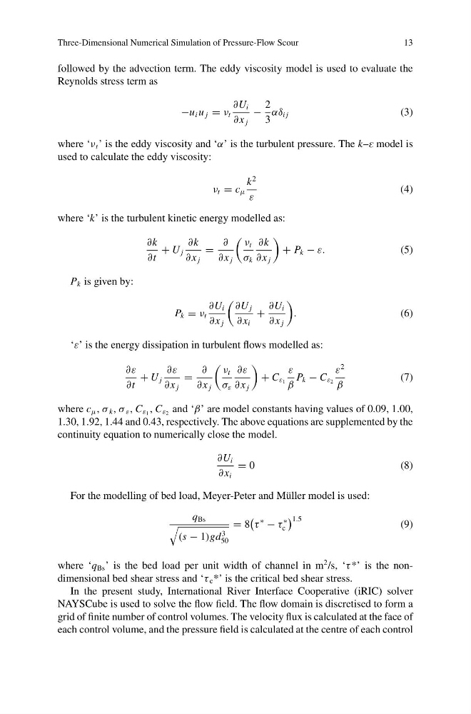
followed by the advection term. The eddy viscosity model is used to evaluate the
Reynolds stress term as
−u i u j = ν t
∂U i
∂ x j
−
2
3
αδ i j
(3)
where ‘ν t ’ is the eddy viscosity and ‘α’ is the turbulent pressure. The k–E model is
used to calculate the eddy viscosity:
ν t = c μ
k
2
ε
(4)
where ‘k’ is the turbulent kinetic energy modelled as:
∂k
∂t
+ U j
∂k
∂ x j
=
∂
∂ x j
ν t
σ k
∂k
∂ x j
+ P k − ε.
(5)
P k is given by:
P k = ν t
∂U i
∂ x j
∂U j
∂ x i
+
∂U i
∂ x j
.
(6)
‘ε’ is the energy dissipation in turbulent flows modelled as:
∂ε
∂t
+ U j
∂ε
∂ x j
=
∂
∂ x j
ν t
σ ε
∂ε
∂ x j
+ C ε 1
ε
β
P k − C ε 2
ε
2
β
(7)
where c μ , σ k , σ ε , C ε 1 , C ε 2 and ‘β’ are model constants having values of 0.09, 1.00,
1.30, 1.92, 1.44 and 0.43, respectively. The above equations are supplemented by the
continuity equation to numerically close the model.
∂U i
∂ x i
= 0
( 8 )
For the modelling of bed load, Meyer-Peter and Müller model is used:
q Bs
(s − 1)gd
3
50
= 8
τ
∗
− τ
∗
c
1.5
(9)
where ‘q Bs ’ is the bed load per unit width of channel in m
2 /s, ‘τ *’ is the nondimensional bed shear stress and ‘τ c *’ is the critical bed shear stress.
In the present study, International River Interface Cooperative (iRIC) solver
NAYSCube is used to solve the flow field. The flow domain is discretised to form a
grid of finite number of control volumes. The velocity flux is calculated at the face of
each control volume, and the pressure field is calculated at the centre of each control
13
followed by the advection term. The eddy viscosity model is used to evaluate the
Reynolds stress term as
−u i u j = ν t
∂U i
∂ x j
−
2
3
αδ i j
(3)
where ‘ν t ’ is the eddy viscosity and ‘α’ is the turbulent pressure. The k–E model is
used to calculate the eddy viscosity:
ν t = c μ
k
2
ε
(4)
where ‘k’ is the turbulent kinetic energy modelled as:
∂k
∂t
+ U j
∂k
∂ x j
=
∂
∂ x j
ν t
σ k
∂k
∂ x j
+ P k − ε.
(5)
P k is given by:
P k = ν t
∂U i
∂ x j
∂U j
∂ x i
+
∂U i
∂ x j
.
(6)
‘ε’ is the energy dissipation in turbulent flows modelled as:
∂ε
∂t
+ U j
∂ε
∂ x j
=
∂
∂ x j
ν t
σ ε
∂ε
∂ x j
+ C ε 1
ε
β
P k − C ε 2
ε
2
β
(7)
where c μ , σ k , σ ε , C ε 1 , C ε 2 and ‘β’ are model constants having values of 0.09, 1.00,
1.30, 1.92, 1.44 and 0.43, respectively. The above equations are supplemented by the
continuity equation to numerically close the model.
∂U i
∂ x i
= 0
( 8 )
For the modelling of bed load, Meyer-Peter and Müller model is used:
q Bs
(s − 1)gd
3
50
= 8
τ
∗
− τ
∗
c
1.5
(9)
where ‘q Bs ’ is the bed load per unit width of channel in m
2 /s, ‘τ *’ is the nondimensional bed shear stress and ‘τ c *’ is the critical bed shear stress.
In the present study, International River Interface Cooperative (iRIC) solver
NAYSCube is used to solve the flow field. The flow domain is discretised to form a
grid of finite number of control volumes. The velocity flux is calculated at the face of
each control volume, and the pressure field is calculated at the centre of each control