

Future Scenarios
It is important to keep in mind that the future climate cannot
be accurately predicted. This can be explained by several
reasons including model uncertainties, uncertainties in scenarios of future greenhouse gas emissions and uncertainties
in natural disturbances, such as volcanism, having a strong
impact on radiative forcing. However, we can try to answer
specific questions: independently of the natural forcings,
how would the climate evolve if greenhouse gas emissions
followed this or that emission pathway? To this end, various
socio-economic scenarios for the evolution of human
activities have been established. Four representative concentration pathways (RCP) scenarios have been selected,
labeled by a value that corresponds approximatively to the
radiative forcing in 2100: RCP2.6, RCP4.5, RCP6.0,
RCP8.5 (top of Fig. 31.11). On one extreme, CO 2 emissions
rapidly stabilize and then decrease down to zero before 2100
for scenario RCP2.6. On the other extreme, CO 2 emissions
continue to grow until 2100 for scenario RCP8.5, which is
for now the most realistic one. CO 2 emissions are mainly
due to the use of fossil fuels (oil, coal, gas) and to the SO 2
emissions from the sulfur contained in these fuels. Mainly
for health reasons, fuels are increasingly purified of sulfur
before use, resulting in a slower increase in CO 2 emissions
(or a faster reduction) than for CO 2 in almost all scenarios.
For the last IPCC exercise (IPCC 2013), the concentrations
of the different gases were calculated from their emissions by
biogeochemical cycle models and by chemical-transport
models for sulfate aerosols. The concentrations of each of
these constituents can then be used to calculate the corresponding radiative forcing. For example, the evolution of the
different forcings from 1860 to 2100 for the RCP8.5 scenarios is shown at the bottom of Fig. 31.11.
The CO 2 Cycle
As described in Chap. 23, the carbon cycle is strongly linked
to the living world. Understanding the roles of the two main
reservoirs, the ocean and the terrestrial biosphere, is therefore crucial to understanding how atmospheric CO 2 will
evolve in the coming decades. The ocean is the largest
carbon reservoir (holding 40 times the atmospheric content)
and can regulate the atmospheric CO 2 concentration by
exchanging CO 2 with the atmosphere. These exchanges
depend largely on the vertical carbon gradient in the ocean:
surface waters are depleted of inorganic carbon and mineral
salts; conversely, the deep ocean is enriched in carbon and
mineral salts. The existence of this vertical gradient is driven
mainly by ocean biology, which establishes a biological
pump and transfers carbon from the surface to the bottom.
Any modification of this pump may ultimately influence the
atmospheric reservoir.
What about anthropogenic disturbances and their impacts
on the carbon cycle? These impacts are manifold: a direct
chemical consequence of the increase in atmospheric CO 2 is
the acidification of the oceans; a thermal consequence of the
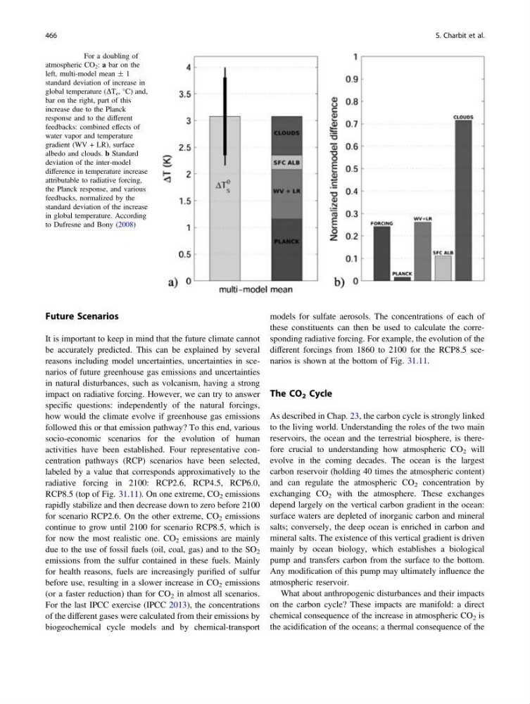
Fig. 31.10 For a doubling of
atmospheric CO 2 : a bar on the
left, multi-model mean ± 1
standard deviation of increase in
global temperature (DT e , °C) and,
bar on the right, part of this
increase due to the Planck
response and to the different
feedbacks: combined effects of
water vapor and temperature
gradient (WV + LR), surface
albedo and clouds. b Standard
deviation of the inter-model
difference in temperature increase
attributable to radiative forcing,
the Planck response, and various
feedbacks, normalized by the
standard deviation of the increase
in global temperature. According
to Dufresne and Bony (2008)
466
S. Charbit et al.
It is important to keep in mind that the future climate cannot
be accurately predicted. This can be explained by several
reasons including model uncertainties, uncertainties in scenarios of future greenhouse gas emissions and uncertainties
in natural disturbances, such as volcanism, having a strong
impact on radiative forcing. However, we can try to answer
specific questions: independently of the natural forcings,
how would the climate evolve if greenhouse gas emissions
followed this or that emission pathway? To this end, various
socio-economic scenarios for the evolution of human
activities have been established. Four representative concentration pathways (RCP) scenarios have been selected,
labeled by a value that corresponds approximatively to the
radiative forcing in 2100: RCP2.6, RCP4.5, RCP6.0,
RCP8.5 (top of Fig. 31.11). On one extreme, CO 2 emissions
rapidly stabilize and then decrease down to zero before 2100
for scenario RCP2.6. On the other extreme, CO 2 emissions
continue to grow until 2100 for scenario RCP8.5, which is
for now the most realistic one. CO 2 emissions are mainly
due to the use of fossil fuels (oil, coal, gas) and to the SO 2
emissions from the sulfur contained in these fuels. Mainly
for health reasons, fuels are increasingly purified of sulfur
before use, resulting in a slower increase in CO 2 emissions
(or a faster reduction) than for CO 2 in almost all scenarios.
For the last IPCC exercise (IPCC 2013), the concentrations
of the different gases were calculated from their emissions by
biogeochemical cycle models and by chemical-transport
models for sulfate aerosols. The concentrations of each of
these constituents can then be used to calculate the corresponding radiative forcing. For example, the evolution of the
different forcings from 1860 to 2100 for the RCP8.5 scenarios is shown at the bottom of Fig. 31.11.
The CO 2 Cycle
As described in Chap. 23, the carbon cycle is strongly linked
to the living world. Understanding the roles of the two main
reservoirs, the ocean and the terrestrial biosphere, is therefore crucial to understanding how atmospheric CO 2 will
evolve in the coming decades. The ocean is the largest
carbon reservoir (holding 40 times the atmospheric content)
and can regulate the atmospheric CO 2 concentration by
exchanging CO 2 with the atmosphere. These exchanges
depend largely on the vertical carbon gradient in the ocean:
surface waters are depleted of inorganic carbon and mineral
salts; conversely, the deep ocean is enriched in carbon and
mineral salts. The existence of this vertical gradient is driven
mainly by ocean biology, which establishes a biological
pump and transfers carbon from the surface to the bottom.
Any modification of this pump may ultimately influence the
atmospheric reservoir.
What about anthropogenic disturbances and their impacts
on the carbon cycle? These impacts are manifold: a direct
chemical consequence of the increase in atmospheric CO 2 is
the acidification of the oceans; a thermal consequence of the
Fig. 31.10 For a doubling of
atmospheric CO 2 : a bar on the
left, multi-model mean ± 1
standard deviation of increase in
global temperature (DT e , °C) and,
bar on the right, part of this
increase due to the Planck
response and to the different
feedbacks: combined effects of
water vapor and temperature
gradient (WV + LR), surface
albedo and clouds. b Standard
deviation of the inter-model
difference in temperature increase
attributable to radiative forcing,
the Planck response, and various
feedbacks, normalized by the
standard deviation of the increase
in global temperature. According
to Dufresne and Bony (2008)
466
S. Charbit et al.