

volume of these glaciers evolved over the centuries. To get
a better idea, climatologists also use graphical representations by painters, and later by photographers. It is thus
clear that after a spread to maximum size at the beginning
of the nineteenth century, the majority of the Alpine glaciers retreated by several kilometers over a century and a
half, with an acceleration of this retreat at the end of the
twentieth century.
Direct Indicators
Historians classify direct observations of climate and meteorology since the year 1000 into several types of historical
phases. These phases qualify the type, abundance and
quality of the information.
Before 1300, these were isolated accounts of extreme
anomalies and natural disasters (Brazdil 2005; Le Roy
Ladurie 1967). These accounts describe in particular the
ravages caused by natural disasters: destruction of crops,
buildings, floods, increased mortality etc. A detailed study of
them, by cross-referencing sources and checking them,
makes it possible to track the chronology of extreme events.
From 1300 to 1500, more or less continuous descriptions
of the character of summers and winters (and to a lesser
extent those of spring and autumn) become available, containing indications of everyday conditions.
From 1500 to 1800, more or less regular descriptions of
monthly or daily conditions start to become available. These
descriptions can be corroborated by records of processions
or rogations organized by the local parishes to end droughts
or avert events that might endanger crops (Le Roy Ladurie
1967).
Between 1680 and 1860, the very first instrumental
measurements appeared. The barometer was invented by
Torricelli and the thermometer by Galileo. The first attempts
to establish international meteorological networks were
made during this time. In France, the first network of systematic observations dates from the reign of Louis XVI. In
1776, Félix Vicq d’Azyr, secretary of the Academy of
Medicine, asked the doctors of the kingdom to record the
temperature of the air three times a day, as well as to write a
summary of the diseases treated during the month. This
initiative was founded on the idea that variations in climate
could have an impact on the health of the population. This
work was maintained for a few decades, and many doctors in
France contributed to the exercise, scrupulously noting
temperatures and diseases. Unfortunately, this directive was
discontinued, and it is not possible to have continuous data.
In addition, the physicians of the day obviously had no
knowledge of meteorology or instrumentation, and not all of
their measurements were reliable.
From 1860 onwards, meteorology was developed within
the framework of national and international networks.
Urbain Le Verrier, who discovered the planet Neptune by
calculation, was also an influential politician of the Second
Empire. Like his astronomer predecessors of the Observatoire de Paris, Cassini, Maraldi and de la Hire, he was also
interested in meteorology and, as a politician, in the strategic
advantage that could be derived from weather forecasting.
Following the disaster of Sevastopol in 1854, when the
Allied fleet was destroyed by a storm, Le Verrier claimed
that it was possible to predict this event through a network of
ad hoc meteorological observations. This marked the birth of
centralized meteorological networks via the telegraph, which
would for a long time be under the control of the army in
most countries in the world.
Statistical Methods for Climate Reconstruction
Methods for obtaining the temperature curves from Fig. 4
are based on statistical regressions between several categories of climate indicators. The general concept behind
reconstructing a hemispheric temperature is to use a set of
indicators (thickness of tree rings, isotopic concentrations,
pollen concentrations, harvest dates etc.) evenly distributed
over the hemisphere. This is called a ‘multi-proxy’ approach
because it uses a mix of several types of climate indicators
(referred to as proxies from now on).
The strategy of these reconstructions (Jones and Mann
2004) is generally in three steps and requires a temperature
dataset with sufficiently good coverage of the globe, hemisphere or well-defined region (e.g., The North Atlantic or the
Equatorial Pacific).
The first step is to determine a small number of general
statistical characteristics (space or time) for recent observations. The best known temperature reconstructions (Mann
et al. 1998) use statistical techniques of decomposition into
principal components (von Storch and Zwiers 2001), however there are alternatives, depending on the distribution of
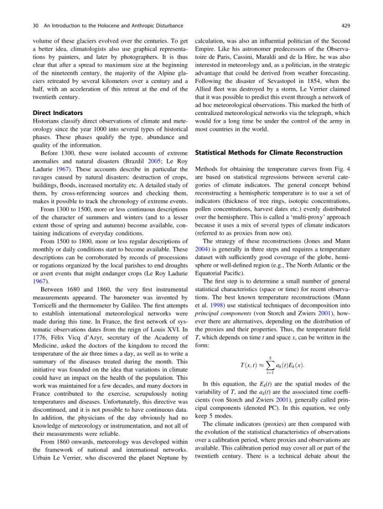
the proxies and their properties. Thus, the temperature field
T, which depends on time t and space x, can be written in the
form:
T x; t
ð Þ %
X 5
t¼1
a k t
ð ÞE k x
ð Þ:
In this equation, the E k (t) are the spatial modes of the
variability of T, and the a k (t) are the associated time coefficients (von Storch and Zwiers 2001), generally called principal components (denoted PC). In this equation, we only
keep 5 modes.
The climate indicators (proxies) are then compared with
the evolution of the statistical characteristics of observations
over a calibration period, where proxies and observations are
available. This calibration period may cover all or part of the
twentieth century. There is a technical debate about the
30 An Introduction to the Holocene and Anthropic Disturbance
429
a better idea, climatologists also use graphical representations by painters, and later by photographers. It is thus
clear that after a spread to maximum size at the beginning
of the nineteenth century, the majority of the Alpine glaciers retreated by several kilometers over a century and a
half, with an acceleration of this retreat at the end of the
twentieth century.
Direct Indicators
Historians classify direct observations of climate and meteorology since the year 1000 into several types of historical
phases. These phases qualify the type, abundance and
quality of the information.
Before 1300, these were isolated accounts of extreme
anomalies and natural disasters (Brazdil 2005; Le Roy
Ladurie 1967). These accounts describe in particular the
ravages caused by natural disasters: destruction of crops,
buildings, floods, increased mortality etc. A detailed study of
them, by cross-referencing sources and checking them,
makes it possible to track the chronology of extreme events.
From 1300 to 1500, more or less continuous descriptions
of the character of summers and winters (and to a lesser
extent those of spring and autumn) become available, containing indications of everyday conditions.
From 1500 to 1800, more or less regular descriptions of
monthly or daily conditions start to become available. These
descriptions can be corroborated by records of processions
or rogations organized by the local parishes to end droughts
or avert events that might endanger crops (Le Roy Ladurie
1967).
Between 1680 and 1860, the very first instrumental
measurements appeared. The barometer was invented by
Torricelli and the thermometer by Galileo. The first attempts
to establish international meteorological networks were
made during this time. In France, the first network of systematic observations dates from the reign of Louis XVI. In
1776, Félix Vicq d’Azyr, secretary of the Academy of
Medicine, asked the doctors of the kingdom to record the
temperature of the air three times a day, as well as to write a
summary of the diseases treated during the month. This
initiative was founded on the idea that variations in climate
could have an impact on the health of the population. This
work was maintained for a few decades, and many doctors in
France contributed to the exercise, scrupulously noting
temperatures and diseases. Unfortunately, this directive was
discontinued, and it is not possible to have continuous data.
In addition, the physicians of the day obviously had no
knowledge of meteorology or instrumentation, and not all of
their measurements were reliable.
From 1860 onwards, meteorology was developed within
the framework of national and international networks.
Urbain Le Verrier, who discovered the planet Neptune by
calculation, was also an influential politician of the Second
Empire. Like his astronomer predecessors of the Observatoire de Paris, Cassini, Maraldi and de la Hire, he was also
interested in meteorology and, as a politician, in the strategic
advantage that could be derived from weather forecasting.
Following the disaster of Sevastopol in 1854, when the
Allied fleet was destroyed by a storm, Le Verrier claimed
that it was possible to predict this event through a network of
ad hoc meteorological observations. This marked the birth of
centralized meteorological networks via the telegraph, which
would for a long time be under the control of the army in
most countries in the world.
Statistical Methods for Climate Reconstruction
Methods for obtaining the temperature curves from Fig. 4
are based on statistical regressions between several categories of climate indicators. The general concept behind
reconstructing a hemispheric temperature is to use a set of
indicators (thickness of tree rings, isotopic concentrations,
pollen concentrations, harvest dates etc.) evenly distributed
over the hemisphere. This is called a ‘multi-proxy’ approach
because it uses a mix of several types of climate indicators
(referred to as proxies from now on).
The strategy of these reconstructions (Jones and Mann
2004) is generally in three steps and requires a temperature
dataset with sufficiently good coverage of the globe, hemisphere or well-defined region (e.g., The North Atlantic or the
Equatorial Pacific).
The first step is to determine a small number of general
statistical characteristics (space or time) for recent observations. The best known temperature reconstructions (Mann
et al. 1998) use statistical techniques of decomposition into
principal components (von Storch and Zwiers 2001), however there are alternatives, depending on the distribution of
the proxies and their properties. Thus, the temperature field
T, which depends on time t and space x, can be written in the
form:
T x; t
ð Þ %
X 5
t¼1
a k t
ð ÞE k x
ð Þ:
In this equation, the E k (t) are the spatial modes of the
variability of T, and the a k (t) are the associated time coefficients (von Storch and Zwiers 2001), generally called principal components (denoted PC). In this equation, we only
keep 5 modes.
The climate indicators (proxies) are then compared with
the evolution of the statistical characteristics of observations
over a calibration period, where proxies and observations are
available. This calibration period may cover all or part of the
twentieth century. There is a technical debate about the
30 An Introduction to the Holocene and Anthropic Disturbance
429