

estimates of the glacial-interglacial amplitude in the center of
Greenland (Dahl-Jensen et al. 1998) and Antarctica (Salamatin
et al. 1998).
Stable Isotopes of Water and Temperature
The most commonly used method to reconstruct variations in
past temperatures at the center of Antarctica and Greenland is
based on analyzing the isotopic composition of the ice. The
study of the abundance of the isotopic forms of water
molecules in precipitations, initiated in the 1950s (Dansgaard
1953), helped to highlight a spatial relationship between
depletion in heavy isotopes and site temperature, a relationship on which the concept of the ‘isotopic thermometer’ is
based. Natural waters, formed mainly of H 2
16 O molecules
(99.7%), also present some rarer stable isotopic forms,
including 0.2% of H 2
18 O and 0.03% of HD
16 O (D represents
deuterium
2 H). The isotopic concentrations are expressed as
the deviation in permil in d notation (dD and d
18 O) against an
international standard, the V-SMOW. At temperate and polar
latitudes, a linear relationship is observed between the isotopic ratios in precipitations today, dD or d
18 O, and the
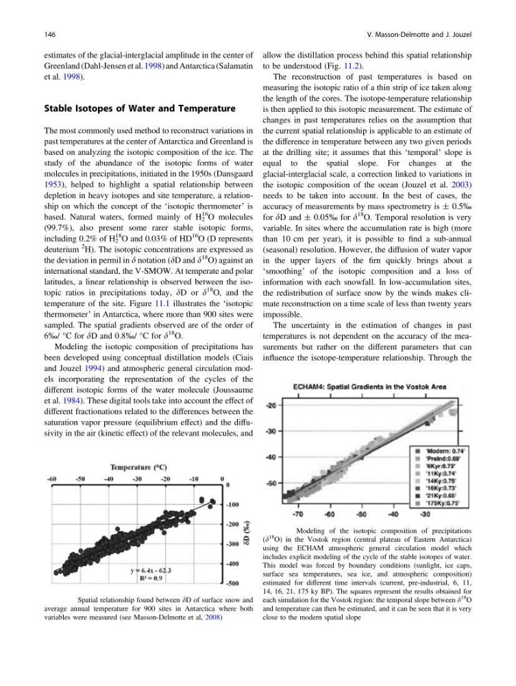
temperature of the site. Figure 11.1 illustrates the ‘isotopic
thermometer’ in Antarctica, where more than 900 sites were
sampled. The spatial gradients observed are of the order of
6‰/ °C for dD and 0.8‰/ °C for d
18 O.
Modeling the isotopic composition of precipitations has
been developed using conceptual distillation models (Ciais
and Jouzel 1994) and atmospheric general circulation models incorporating the representation of the cycles of the
different isotopic forms of the water molecule (Joussaume
et al. 1984). These digital tools take into account the effect of
different fractionations related to the differences between the
saturation vapor pressure (equilibrium effect) and the diffusivity in the air (kinetic effect) of the relevant molecules, and
allow the distillation process behind this spatial relationship
to be understood (Fig. 11.2).
The reconstruction of past temperatures is based on
measuring the isotopic ratio of a thin strip of ice taken along
the length of the cores. The isotope-temperature relationship
is then applied to this isotopic measurement. The estimate of
changes in past temperatures relies on the assumption that
the current spatial relationship is applicable to an estimate of
the difference in temperature between any two given periods
at the drilling site; it assumes that this ‘temporal’ slope is
equal to the spatial slope. For changes at the
glacial-interglacial scale, a correction linked to variations in
the isotopic composition of the ocean (Jouzel et al. 2003)
needs to be taken into account. In the best of cases, the
accuracy of measurements by mass spectrometry is ± 0.5‰
for dD and ± 0.05‰ for d
18 O. Temporal resolution is very
variable. In sites where the accumulation rate is high (more
than 10 cm per year), it is possible to find a sub-annual
(seasonal) resolution. However, the diffusion of water vapor
in the upper layers of the firn quickly brings about a
‘smoothing’ of the isotopic composition and a loss of
information with each snowfall. In low-accumulation sites,
the redistribution of surface snow by the winds makes climate reconstruction on a time scale of less than twenty years
impossible.
The uncertainty in the estimation of changes in past
temperatures is not dependent on the accuracy of the measurements but rather on the different parameters that can
influence the isotope-temperature relationship. Through the
Fig. 11.1 Spatial relationship found between dD of surface snow and
average annual temperature for 900 sites in Antarctica where both
variables were measured (see Masson-Delmotte et al, 2008)
Fig. 11.2 Modeling of the isotopic composition of precipitations
(d
18
O) in the Vostok region (central plateau of Eastern Antarctica)
using the ECHAM atmospheric general circulation model which
includes explicit modeling of the cycle of the stable isotopes of water.
This model was forced by boundary conditions (sunlight, ice caps,
surface sea temperatures, sea ice, and atmospheric composition)
estimated for different time intervals (current, pre-industrial, 6, 11,
14, 16, 21, 175 ky BP). The squares represent the results obtained for
each simulation for the Vostok region: the temporal slope between d
18
O
and temperature can then be estimated, and it can be seen that it is very
close to the modern spatial slope
146
V. Masson-Delmotte and J. Jouzel
Greenland (Dahl-Jensen et al. 1998) and Antarctica (Salamatin
et al. 1998).
Stable Isotopes of Water and Temperature
The most commonly used method to reconstruct variations in
past temperatures at the center of Antarctica and Greenland is
based on analyzing the isotopic composition of the ice. The
study of the abundance of the isotopic forms of water
molecules in precipitations, initiated in the 1950s (Dansgaard
1953), helped to highlight a spatial relationship between
depletion in heavy isotopes and site temperature, a relationship on which the concept of the ‘isotopic thermometer’ is
based. Natural waters, formed mainly of H 2
16 O molecules
(99.7%), also present some rarer stable isotopic forms,
including 0.2% of H 2
18 O and 0.03% of HD
16 O (D represents
deuterium
2 H). The isotopic concentrations are expressed as
the deviation in permil in d notation (dD and d
18 O) against an
international standard, the V-SMOW. At temperate and polar
latitudes, a linear relationship is observed between the isotopic ratios in precipitations today, dD or d
18 O, and the
temperature of the site. Figure 11.1 illustrates the ‘isotopic
thermometer’ in Antarctica, where more than 900 sites were
sampled. The spatial gradients observed are of the order of
6‰/ °C for dD and 0.8‰/ °C for d
18 O.
Modeling the isotopic composition of precipitations has
been developed using conceptual distillation models (Ciais
and Jouzel 1994) and atmospheric general circulation models incorporating the representation of the cycles of the
different isotopic forms of the water molecule (Joussaume
et al. 1984). These digital tools take into account the effect of
different fractionations related to the differences between the
saturation vapor pressure (equilibrium effect) and the diffusivity in the air (kinetic effect) of the relevant molecules, and
allow the distillation process behind this spatial relationship
to be understood (Fig. 11.2).
The reconstruction of past temperatures is based on
measuring the isotopic ratio of a thin strip of ice taken along
the length of the cores. The isotope-temperature relationship
is then applied to this isotopic measurement. The estimate of
changes in past temperatures relies on the assumption that
the current spatial relationship is applicable to an estimate of
the difference in temperature between any two given periods
at the drilling site; it assumes that this ‘temporal’ slope is
equal to the spatial slope. For changes at the
glacial-interglacial scale, a correction linked to variations in
the isotopic composition of the ocean (Jouzel et al. 2003)
needs to be taken into account. In the best of cases, the
accuracy of measurements by mass spectrometry is ± 0.5‰
for dD and ± 0.05‰ for d
18 O. Temporal resolution is very
variable. In sites where the accumulation rate is high (more
than 10 cm per year), it is possible to find a sub-annual
(seasonal) resolution. However, the diffusion of water vapor
in the upper layers of the firn quickly brings about a
‘smoothing’ of the isotopic composition and a loss of
information with each snowfall. In low-accumulation sites,
the redistribution of surface snow by the winds makes climate reconstruction on a time scale of less than twenty years
impossible.
The uncertainty in the estimation of changes in past
temperatures is not dependent on the accuracy of the measurements but rather on the different parameters that can
influence the isotope-temperature relationship. Through the
Fig. 11.1 Spatial relationship found between dD of surface snow and
average annual temperature for 900 sites in Antarctica where both
variables were measured (see Masson-Delmotte et al, 2008)
Fig. 11.2 Modeling of the isotopic composition of precipitations
(d
18
O) in the Vostok region (central plateau of Eastern Antarctica)
using the ECHAM atmospheric general circulation model which
includes explicit modeling of the cycle of the stable isotopes of water.
This model was forced by boundary conditions (sunlight, ice caps,
surface sea temperatures, sea ice, and atmospheric composition)
estimated for different time intervals (current, pre-industrial, 6, 11,
14, 16, 21, 175 ky BP). The squares represent the results obtained for
each simulation for the Vostok region: the temporal slope between d
18
O
and temperature can then be estimated, and it can be seen that it is very
close to the modern spatial slope
146
V. Masson-Delmotte and J. Jouzel