

46
S. Droulias and L. Bougas
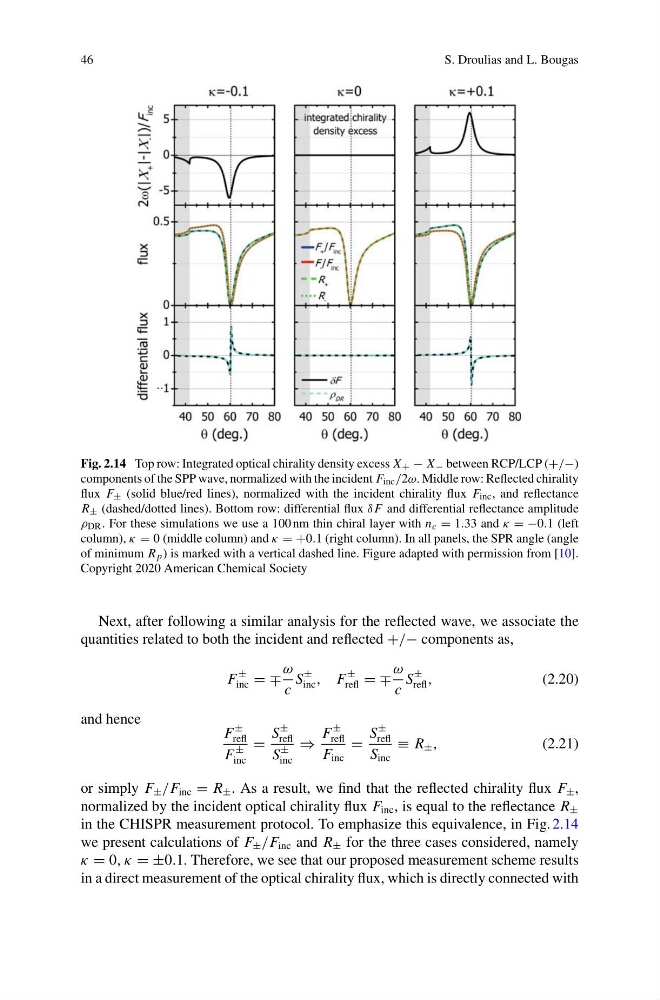
Fig. 2.14 Top row: Integrated optical chirality density excess X + − X − between RCP/LCP (+/−)
components of the SPP wave, normalized with the incident F inc /2ω. Middle row: Reflected chirality
flux F ± (solid blue/red lines), normalized with the incident chirality flux F inc , and reflectance
R ± (dashed/dotted lines). Bottom row: differential flux δ F and differential reflectance amplitude
ρ DR . For these simulations we use a 100 nm thin chiral layer with n c = 1.33 and κ = −0.1 (left
column), κ = 0 (middle column) and κ = +0.1 (right column). In all panels, the SPR angle (angle
of minimum R p ) is marked with a vertical dashed line. Figure adapted with permission from [10].
Copyright 2020 American Chemical Society
Next, after following a similar analysis for the reflected wave, we associate the
quantities related to both the incident and reflected +/− components as,
F
±
inc = ∓
ω
c
S
±
inc , F
±
refl = ∓
ω
c
S
±
refl ,
(2.20)
and hence
F
±
refl
F
±
inc
=
S
±
refl
S
±
inc
⇒
F
±
refl
F inc
=
S
±
refl
S inc
≡ R ± ,
(2.21)
or simply F ± /F inc = R ± . As a result, we find that the reflected chirality flux F ± ,
normalized by the incident optical chirality flux F inc , is equal to the reflectance R ±
in the CHISPR measurement protocol. To emphasize this equivalence, in Fig. 2.14
we present calculations of F ± /F inc and R ± for the three cases considered, namely
κ = 0, κ = ±0.1. Therefore, we see that our proposed measurement scheme results
in a direct measurement of the optical chirality flux, which is directly connected with
S. Droulias and L. Bougas
Fig. 2.14 Top row: Integrated optical chirality density excess X + − X − between RCP/LCP (+/−)
components of the SPP wave, normalized with the incident F inc /2ω. Middle row: Reflected chirality
flux F ± (solid blue/red lines), normalized with the incident chirality flux F inc , and reflectance
R ± (dashed/dotted lines). Bottom row: differential flux δ F and differential reflectance amplitude
ρ DR . For these simulations we use a 100 nm thin chiral layer with n c = 1.33 and κ = −0.1 (left
column), κ = 0 (middle column) and κ = +0.1 (right column). In all panels, the SPR angle (angle
of minimum R p ) is marked with a vertical dashed line. Figure adapted with permission from [10].
Copyright 2020 American Chemical Society
Next, after following a similar analysis for the reflected wave, we associate the
quantities related to both the incident and reflected +/− components as,
F
±
inc = ∓
ω
c
S
±
inc , F
±
refl = ∓
ω
c
S
±
refl ,
(2.20)
and hence
F
±
refl
F
±
inc
=
S
±
refl
S
±
inc
⇒
F
±
refl
F inc
=
S
±
refl
S inc
≡ R ± ,
(2.21)
or simply F ± /F inc = R ± . As a result, we find that the reflected chirality flux F ± ,
normalized by the incident optical chirality flux F inc , is equal to the reflectance R ±
in the CHISPR measurement protocol. To emphasize this equivalence, in Fig. 2.14
we present calculations of F ± /F inc and R ± for the three cases considered, namely
κ = 0, κ = ±0.1. Therefore, we see that our proposed measurement scheme results
in a direct measurement of the optical chirality flux, which is directly connected with