

19 Magnetoelectric Near Fields
537
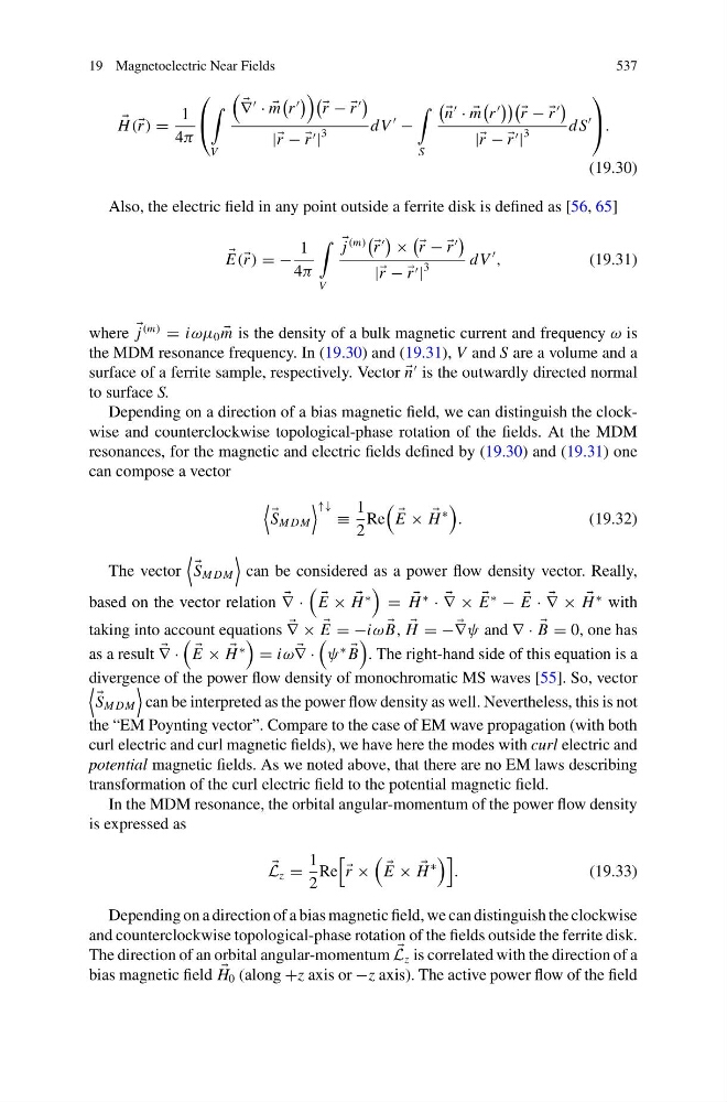
H ( r ) =
1
4π
⎛
⎝
V
∇
· ·
m
r
r − −
r
| r − −
r |
3
dV
−
S
n
· ·
m
r
r − −
r
| r − −
r |
3
d S
⎞
⎠ .
(19.30)
Also, the electric field in any point outside a ferrite disk is defined as [56, 65]
E( r ) = −
1
4π
V
j
(m)
r
×
r − −
r
| r − −
r |
3
dV
,
(19.31)
where j
(m)
= iωμ 0
m is the density of a bulk magnetic current and frequency ω is
the MDM resonance frequency. In (19.30) and (19.31), V and S are a volume and a
surface of a ferrite sample, respectively. Vector
n
is the outwardly directed normal
to surface S.
Depending on a direction of a bias magnetic field, we can distinguish the clockwise and counterclockwise topological-phase rotation of the fields. At the MDM
resonances, for the magnetic and electric fields defined by (19.30) and (19.31) one
can compose a vector
S M DM
↑↓ ≡
1
2
Re
E ×
H
∗
.
(19.32)
The vector
S M DM
can be considered as a power flow density vector. Really,
based on the vector relation
∇ ·
E ×
H
∗
=
H
∗
·
∇ ×
E
∗
−
E ·
∇ ×
H
∗ with
taking into account equations
∇ ×
E = −iω
B,
H = −
∇ψ and ∇ ·
B = 0, one has
as a result
∇ ·
E ×
H
∗
= iω
∇ ·
ψ
∗
B
. The right-hand side of this equation is a
divergence of the power flow density of monochromatic MS waves [55]. So, vector
S M DM
can be interpreted as the power flow density as well. Nevertheless, this is not
the “EM Poynting vector”. Compare to the case of EM wave propagation (with both
curl electric and curl magnetic fields), we have here the modes with curl electric and
potential magnetic fields. As we noted above, that there are no EM laws describing
transformation of the curl electric field to the potential magnetic field.
In the MDM resonance, the orbital angular-momentum of the power flow density
is expressed as
L z =
1
2
Re
r ×
E ×
H
∗
.
(19.33)
Depending on a direction of a bias magnetic field, we can distinguish the clockwise
and counterclockwise topological-phase rotation of the fields outside the ferrite disk.
The direction of an orbital angular-momentum
L z is correlated with the direction of a
bias magnetic field
H 0 (along +z axis or −z axis). The active power flow of the field
537
H ( r ) =
1
4π
⎛
⎝
V
∇
· ·
m
r
r − −
r
| r − −
r |
3
dV
−
S
n
· ·
m
r
r − −
r
| r − −
r |
3
d S
⎞
⎠ .
(19.30)
Also, the electric field in any point outside a ferrite disk is defined as [56, 65]
E( r ) = −
1
4π
V
j
(m)
r
×
r − −
r
| r − −
r |
3
dV
,
(19.31)
where j
(m)
= iωμ 0
m is the density of a bulk magnetic current and frequency ω is
the MDM resonance frequency. In (19.30) and (19.31), V and S are a volume and a
surface of a ferrite sample, respectively. Vector
n
is the outwardly directed normal
to surface S.
Depending on a direction of a bias magnetic field, we can distinguish the clockwise and counterclockwise topological-phase rotation of the fields. At the MDM
resonances, for the magnetic and electric fields defined by (19.30) and (19.31) one
can compose a vector
S M DM
↑↓ ≡
1
2
Re
E ×
H
∗
.
(19.32)
The vector
S M DM
can be considered as a power flow density vector. Really,
based on the vector relation
∇ ·
E ×
H
∗
=
H
∗
·
∇ ×
E
∗
−
E ·
∇ ×
H
∗ with
taking into account equations
∇ ×
E = −iω
B,
H = −
∇ψ and ∇ ·
B = 0, one has
as a result
∇ ·
E ×
H
∗
= iω
∇ ·
ψ
∗
B
. The right-hand side of this equation is a
divergence of the power flow density of monochromatic MS waves [55]. So, vector
S M DM
can be interpreted as the power flow density as well. Nevertheless, this is not
the “EM Poynting vector”. Compare to the case of EM wave propagation (with both
curl electric and curl magnetic fields), we have here the modes with curl electric and
potential magnetic fields. As we noted above, that there are no EM laws describing
transformation of the curl electric field to the potential magnetic field.
In the MDM resonance, the orbital angular-momentum of the power flow density
is expressed as
L z =
1
2
Re
r ×
E ×
H
∗
.
(19.33)
Depending on a direction of a bias magnetic field, we can distinguish the clockwise
and counterclockwise topological-phase rotation of the fields outside the ferrite disk.
The direction of an orbital angular-momentum
L z is correlated with the direction of a
bias magnetic field
H 0 (along +z axis or −z axis). The active power flow of the field