

19 Magnetoelectric Near Fields
535
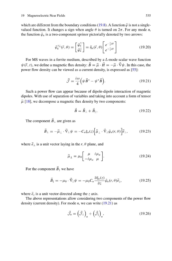
which are different from the boundary conditions (19.8). A function ˜
ϕ is not a singlevalued function. It changes a sign when angle θ is turned on 2π . For any mode n,
the function ˜
ϕ n is a two-component sprinor pictorially denoted by two arrows:
˜
ϕ
↑↓
n ( r , θ) =
˜
ϕ
↑
n
˜
ϕ
↓
n
= ˜
η n ( r , θ)
e
−
1
2 iθ
e
+
1
2 iθ
(19.20)
For MS waves in a ferrite medium, described by a L-mode scalar wave function
ψ( r , t), we define a magnetic flux density:
B =
↔
μ ·
H = −
↔
μ ·
∇ψ. In this case, the
power flow density can be viewed as a current density, is expressed as [55]:
J =
iω
4
ψ
B
∗
− ψ
∗
B
.
(19.21)
Such a power flow can appear because of dipole-dipole interaction of magnetic
dipoles. With use of separation of variables and taking into account a form of tensor
↔
μ [18], we decompose a magnetic flux density by two components:
B =
B ⊥ +
B || .
(19.22)
The component
B ⊥ are given as
B ⊥ = −
↔
μ ⊥ ·
∇ ⊥ ψ = −C n ξ n (z)
↔
μ ⊥ ·
∇ ⊥ ˜
ϕ n (r, θ)
e ⊥ ,
(19.23)
where
e ⊥ is a unit vector laying in the r, θ plane, and
↔
μ ⊥ = μ 0
μ iμ a
−iμ a μ
.
(19.24)
For the component
B we have
B = −μ 0 ·
∇ || ψ = −μ 0 C n
∂ξ n (z)
∂z
˜
ϕ n (r, θ) e z ,
(19.25)
where
e z is a unit vector directed along the z axis.
The above representations allow considering two components of the power flow
density (current density). For mode n, we can write (19.21) as
J n =
J ⊥
n
+
J
n
,
(19.26)
535
which are different from the boundary conditions (19.8). A function ˜
ϕ is not a singlevalued function. It changes a sign when angle θ is turned on 2π . For any mode n,
the function ˜
ϕ n is a two-component sprinor pictorially denoted by two arrows:
˜
ϕ
↑↓
n ( r , θ) =
˜
ϕ
↑
n
˜
ϕ
↓
n
= ˜
η n ( r , θ)
e
−
1
2 iθ
e
+
1
2 iθ
(19.20)
For MS waves in a ferrite medium, described by a L-mode scalar wave function
ψ( r , t), we define a magnetic flux density:
B =
↔
μ ·
H = −
↔
μ ·
∇ψ. In this case, the
power flow density can be viewed as a current density, is expressed as [55]:
J =
iω
4
ψ
B
∗
− ψ
∗
B
.
(19.21)
Such a power flow can appear because of dipole-dipole interaction of magnetic
dipoles. With use of separation of variables and taking into account a form of tensor
↔
μ [18], we decompose a magnetic flux density by two components:
B =
B ⊥ +
B || .
(19.22)
The component
B ⊥ are given as
B ⊥ = −
↔
μ ⊥ ·
∇ ⊥ ψ = −C n ξ n (z)
↔
μ ⊥ ·
∇ ⊥ ˜
ϕ n (r, θ)
e ⊥ ,
(19.23)
where
e ⊥ is a unit vector laying in the r, θ plane, and
↔
μ ⊥ = μ 0
μ iμ a
−iμ a μ
.
(19.24)
For the component
B we have
B = −μ 0 ·
∇ || ψ = −μ 0 C n
∂ξ n (z)
∂z
˜
ϕ n (r, θ) e z ,
(19.25)
where
e z is a unit vector directed along the z axis.
The above representations allow considering two components of the power flow
density (current density). For mode n, we can write (19.21) as
J n =
J ⊥
n
+
J
n
,
(19.26)