

17 Axion Electrodynamics in Magnetoelectric Media
469
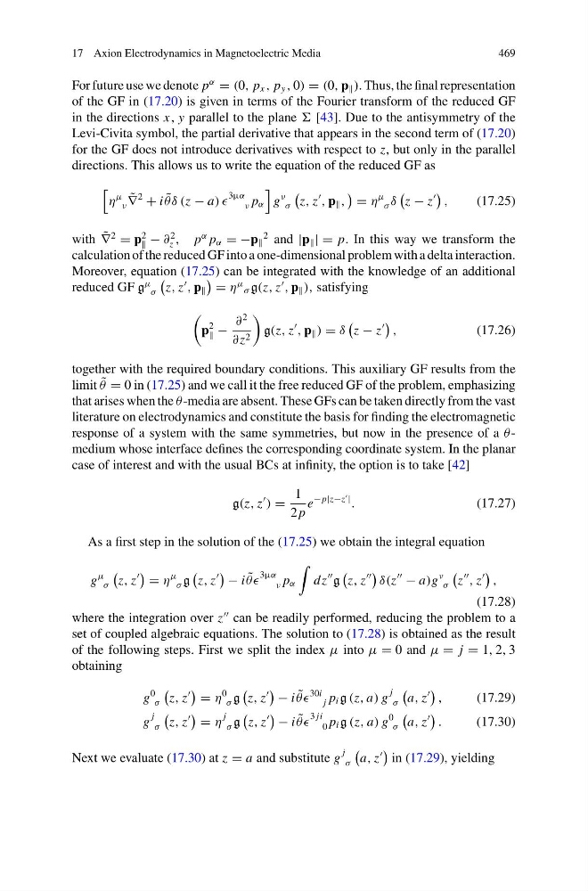
For future use we denote p
α
= (0, p x , p y , 0) = (0, p ). Thus, the final representation
of the GF in (17.20) is given in terms of the Fourier transform of the reduced GF
in the directions x, y parallel to the plane [43]. Due to the antisymmetry of the
Levi-Civita symbol, the partial derivative that appears in the second term of (17.20)
for the GF does not introduce derivatives with respect to z, but only in the parallel
directions. This allows us to write the equation of the reduced GF as
η
μ
ν
˜
∇
2
+ i ˜
θδ (z − a)
3µα
ν p α
g
ν
σ
z, z
, p ,
= η
μ
σ δ
z − z
,
(17.25)
with ˜
∇
2
= p
2
− ∂
2
z , p
α p α = −p
2 and |p | = p. In this way we transform the
calculation of the reduced GF into a one-dimensional problem with a delta interaction.
Moreover, equation (17.25) can be integrated with the knowledge of an additional
reduced GF g
μ σ
z, z
, p
= η
μ σ g(z, z
, p ), satisfying
p
2
−
∂
2
∂z 2
g(z, z
, p ) = δ
z − z
,
(17.26)
together with the required boundary conditions. This auxiliary GF results from the
limit ˜
θ = 0 in (17.25) and we call it the free reduced GF of the problem, emphasizing
that arises when the θ -media are absent. These GFs can be taken directly from the vast
literature on electrodynamics and constitute the basis for finding the electromagnetic
response of a system with the same symmetries, but now in the presence of a θ -
medium whose interface defines the corresponding coordinate system. In the planar
case of interest and with the usual BCs at infinity, the option is to take [42]
g(z, z
) =
1
2 p
e
− p|z−z
|
.
(17.27)
As a first step in the solution of the (17.25) we obtain the integral equation
g
μ
σ
z, z
= η
μ
σ g
z, z
− i ˜
θθ
3µα
ν p α
dz
g
z, z
δ(z
− a)g
ν
σ
z
, z
,
(17.28)
where the integration over z
can be readily performed, reducing the problem to a
set of coupled algebraic equations. The solution to (17.28) is obtained as the result
of the following steps. First we split the index μ into μ = 0 and μ = j = 1, 2, 3
obtaining
g
0
σ
z, z
= η
0
σ g
z, z
− i ˜
θθ
30i
j p i g (z, a) g
j
σ
a, z
,
(17.29)
g
j
σ
z, z
= η
j
σ g
z, z
− i ˜
θθ
3 ji
0 p i g (z, a) g
0
σ
a, z
.
(17.30)
Next we evaluate (17.30) at z = a and substitute g
j
σ
a, z
in (17.29), yielding
469
For future use we denote p
α
= (0, p x , p y , 0) = (0, p ). Thus, the final representation
of the GF in (17.20) is given in terms of the Fourier transform of the reduced GF
in the directions x, y parallel to the plane [43]. Due to the antisymmetry of the
Levi-Civita symbol, the partial derivative that appears in the second term of (17.20)
for the GF does not introduce derivatives with respect to z, but only in the parallel
directions. This allows us to write the equation of the reduced GF as
η
μ
ν
˜
∇
2
+ i ˜
θδ (z − a)
3µα
ν p α
g
ν
σ
z, z
, p ,
= η
μ
σ δ
z − z
,
(17.25)
with ˜
∇
2
= p
2
− ∂
2
z , p
α p α = −p
2 and |p | = p. In this way we transform the
calculation of the reduced GF into a one-dimensional problem with a delta interaction.
Moreover, equation (17.25) can be integrated with the knowledge of an additional
reduced GF g
μ σ
z, z
, p
= η
μ σ g(z, z
, p ), satisfying
p
2
−
∂
2
∂z 2
g(z, z
, p ) = δ
z − z
,
(17.26)
together with the required boundary conditions. This auxiliary GF results from the
limit ˜
θ = 0 in (17.25) and we call it the free reduced GF of the problem, emphasizing
that arises when the θ -media are absent. These GFs can be taken directly from the vast
literature on electrodynamics and constitute the basis for finding the electromagnetic
response of a system with the same symmetries, but now in the presence of a θ -
medium whose interface defines the corresponding coordinate system. In the planar
case of interest and with the usual BCs at infinity, the option is to take [42]
g(z, z
) =
1
2 p
e
− p|z−z
|
.
(17.27)
As a first step in the solution of the (17.25) we obtain the integral equation
g
μ
σ
z, z
= η
μ
σ g
z, z
− i ˜
θθ
3µα
ν p α
dz
g
z, z
δ(z
− a)g
ν
σ
z
, z
,
(17.28)
where the integration over z
can be readily performed, reducing the problem to a
set of coupled algebraic equations. The solution to (17.28) is obtained as the result
of the following steps. First we split the index μ into μ = 0 and μ = j = 1, 2, 3
obtaining
g
0
σ
z, z
= η
0
σ g
z, z
− i ˜
θθ
30i
j p i g (z, a) g
j
σ
a, z
,
(17.29)
g
j
σ
z, z
= η
j
σ g
z, z
− i ˜
θθ
3 ji
0 p i g (z, a) g
0
σ
a, z
.
(17.30)
Next we evaluate (17.30) at z = a and substitute g
j
σ
a, z
in (17.29), yielding