

466
A. Martín-Ruiz et al.
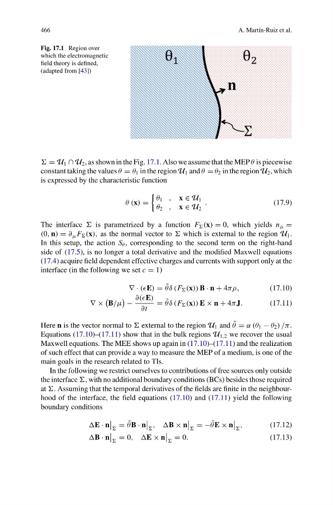
Fig. 17.1 Region over
which the electromagnetic
field theory is defined,
(adapted from [43])
= U 1 ∩ U 2 , as shown in the Fig. 17.1. Also we assume that the MEP θ is piecewise
constant taking the values θ = θ 1 in the region U 1 and θ = θ 2 in the region U 2 , which
is expressed by the characteristic function
θ (x) =
θ 1 , x ∈ U 1
θ 2 , x ∈ U 2
.
(17.9)
The interface is parametrized by a function F (x) = 0, which yields n μ =
(0, n) = ∂ μ F (x), as the normal vector to which is external to the region U 1 .
In this setup, the action S θ , corresponding to the second term on the right-hand
side of (17.5), is no longer a total derivative and the modified Maxwell equations
(17.4) acquire field dependent effective charges and currents with support only at the
interface (in the following we set c = 1)
∇ · ((E) = ˜
θδ (F (x)) B · n + 4πρ,
(17.10)
∇ ×
B/μ
−
∂((E)
∂t
= ˜
θδ (F (x)) E × n + 4π J.
(17.11)
Here n is the vector normal to external to the region U 1 and ˜
θ = α (θ 1 − θ 2 ) /π .
Equations (17.10)–(17.11) show that in the bulk regions U 1,2 we recover the usual
Maxwell equations. The MEE shows up again in (17.10)–(17.11) and the realization
of such effect that can provide a way to measure the MEP of a medium, is one of the
main goals in the research related to TIs.
In the following we restrict ourselves to contributions of free sources only outside
the interface , with no additional boundary conditions (BCs) besides those required
at . Assuming that the temporal derivatives of the fields are finite in the neighbourhood of the interface, the field equations (17.10) and (17.11) yield the following
boundary conditions
E · n
= ˜
θ B · n
, ,B × n
= − ˜
θ E × n
,
(17.12)
B · n
= 0, ,E × n
= 0.
(17.13)
A. Martín-Ruiz et al.
Fig. 17.1 Region over
which the electromagnetic
field theory is defined,
(adapted from [43])
= U 1 ∩ U 2 , as shown in the Fig. 17.1. Also we assume that the MEP θ is piecewise
constant taking the values θ = θ 1 in the region U 1 and θ = θ 2 in the region U 2 , which
is expressed by the characteristic function
θ (x) =
θ 1 , x ∈ U 1
θ 2 , x ∈ U 2
.
(17.9)
The interface is parametrized by a function F (x) = 0, which yields n μ =
(0, n) = ∂ μ F (x), as the normal vector to which is external to the region U 1 .
In this setup, the action S θ , corresponding to the second term on the right-hand
side of (17.5), is no longer a total derivative and the modified Maxwell equations
(17.4) acquire field dependent effective charges and currents with support only at the
interface (in the following we set c = 1)
∇ · ((E) = ˜
θδ (F (x)) B · n + 4πρ,
(17.10)
∇ ×
B/μ
−
∂((E)
∂t
= ˜
θδ (F (x)) E × n + 4π J.
(17.11)
Here n is the vector normal to external to the region U 1 and ˜
θ = α (θ 1 − θ 2 ) /π .
Equations (17.10)–(17.11) show that in the bulk regions U 1,2 we recover the usual
Maxwell equations. The MEE shows up again in (17.10)–(17.11) and the realization
of such effect that can provide a way to measure the MEP of a medium, is one of the
main goals in the research related to TIs.
In the following we restrict ourselves to contributions of free sources only outside
the interface , with no additional boundary conditions (BCs) besides those required
at . Assuming that the temporal derivatives of the fields are finite in the neighbourhood of the interface, the field equations (17.10) and (17.11) yield the following
boundary conditions
E · n
= ˜
θ B · n
, ,B × n
= − ˜
θ E × n
,
(17.12)
B · n
= 0, ,E × n
= 0.
(17.13)