

450
L. Shen et al.
As shown in Fig. 16.6a, the magnetic anisotropy gradient (dK/dx = 100 GJ/m
4 ) is
assumed to be induced by applying a voltage to the sample with a wedged insulating
layer. Taking such an anisotropy gradient, i.e., dK/dx = 100 GJ/m
4 , the motion
of the antiferromagnetic skyrmion is simulated by solving the dynamic equation
of antiferromagnet, and the time evolution of the skyrmion speed v x is shown in
Fig. 16.6b. We can see that the antiferromagnetic skyrmion is first accelerated to 450
m/s in 0.2 ns and then its speed increases slowly to 504 m/s by t = 0.5 ns [35]. The
speed cannot reach a constant value, as the decreasing magnetic anisotropy K gives
rise to the change of the skyrmion size. Namely, when the skyrmion moves in the
positive x direction, the decreasing K results in the increase of the skyrmion size,
so that the skyrmion speed will increase slowly. Fig. 16.6c shows the top view of
the skyrmion motion, from which we can see that the radius of the skyrmion at t =
0.5 ns is larger than that of the initial state. Such an effect also exists in the case of
ferromagnetic skyrmions driven by an anisotropy gradient, as reported by Tomasello
et al. [62].
On the other hand, in antiferromagnetic systems, the magnetic moments of sublattices are compensated, so that the antiferromagnetic skyrmions do not show the
skyrmion Hall effect [29, 30] due to zero net Magnus force. However, for ferromagnetic skyrmions, there is a transverse drift, i.e., the skyrmion Hall effect. Therefore, the motion behaviors of antiferromagnetic skyrmions driven by an anisotropy
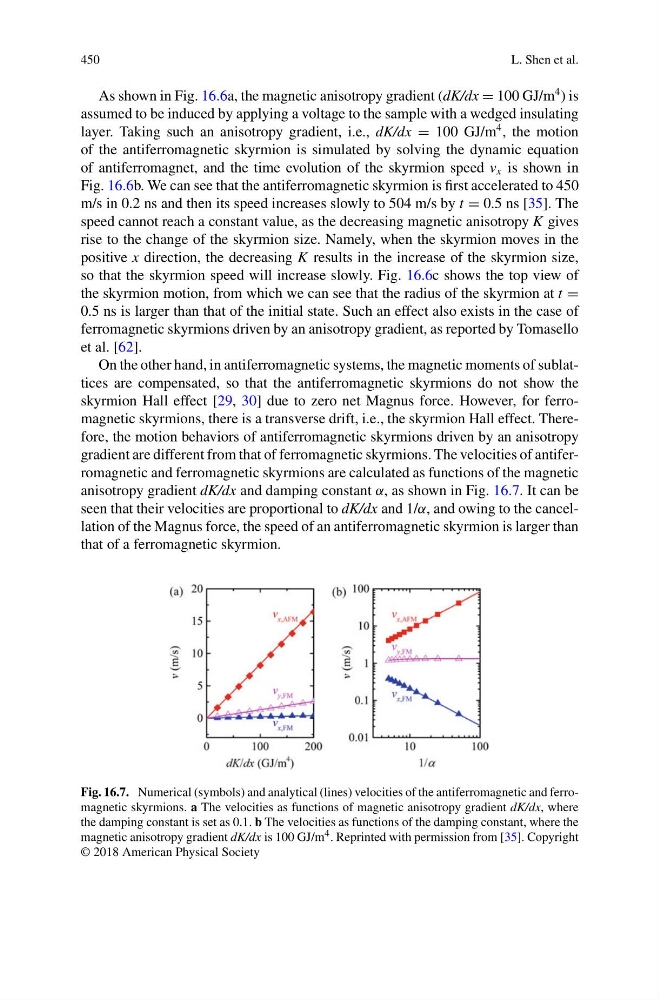
gradient are different from that of ferromagnetic skyrmions. The velocities of antiferromagnetic and ferromagnetic skyrmions are calculated as functions of the magnetic
anisotropy gradient dK/dx and damping constant α, as shown in Fig. 16.7. It can be
seen that their velocities are proportional to dK/dx and 1/α, and owing to the cancellation of the Magnus force, the speed of an antiferromagnetic skyrmion is larger than
that of a ferromagnetic skyrmion.
Fig. 16.7. Numerical (symbols) and analytical (lines) velocities of the antiferromagnetic and ferromagnetic skyrmions. a The velocities as functions of magnetic anisotropy gradient dK/dx, where
the damping constant is set as 0.1. b The velocities as functions of the damping constant, where the
magnetic anisotropy gradient dK/dx is 100 GJ/m 4 . Reprinted with permission from [35]. Copyright
© 2018 American Physical Society
L. Shen et al.
As shown in Fig. 16.6a, the magnetic anisotropy gradient (dK/dx = 100 GJ/m
4 ) is
assumed to be induced by applying a voltage to the sample with a wedged insulating
layer. Taking such an anisotropy gradient, i.e., dK/dx = 100 GJ/m
4 , the motion
of the antiferromagnetic skyrmion is simulated by solving the dynamic equation
of antiferromagnet, and the time evolution of the skyrmion speed v x is shown in
Fig. 16.6b. We can see that the antiferromagnetic skyrmion is first accelerated to 450
m/s in 0.2 ns and then its speed increases slowly to 504 m/s by t = 0.5 ns [35]. The
speed cannot reach a constant value, as the decreasing magnetic anisotropy K gives
rise to the change of the skyrmion size. Namely, when the skyrmion moves in the
positive x direction, the decreasing K results in the increase of the skyrmion size,
so that the skyrmion speed will increase slowly. Fig. 16.6c shows the top view of
the skyrmion motion, from which we can see that the radius of the skyrmion at t =
0.5 ns is larger than that of the initial state. Such an effect also exists in the case of
ferromagnetic skyrmions driven by an anisotropy gradient, as reported by Tomasello
et al. [62].
On the other hand, in antiferromagnetic systems, the magnetic moments of sublattices are compensated, so that the antiferromagnetic skyrmions do not show the
skyrmion Hall effect [29, 30] due to zero net Magnus force. However, for ferromagnetic skyrmions, there is a transverse drift, i.e., the skyrmion Hall effect. Therefore, the motion behaviors of antiferromagnetic skyrmions driven by an anisotropy
gradient are different from that of ferromagnetic skyrmions. The velocities of antiferromagnetic and ferromagnetic skyrmions are calculated as functions of the magnetic
anisotropy gradient dK/dx and damping constant α, as shown in Fig. 16.7. It can be
seen that their velocities are proportional to dK/dx and 1/α, and owing to the cancellation of the Magnus force, the speed of an antiferromagnetic skyrmion is larger than
that of a ferromagnetic skyrmion.
Fig. 16.7. Numerical (symbols) and analytical (lines) velocities of the antiferromagnetic and ferromagnetic skyrmions. a The velocities as functions of magnetic anisotropy gradient dK/dx, where
the damping constant is set as 0.1. b The velocities as functions of the damping constant, where the
magnetic anisotropy gradient dK/dx is 100 GJ/m 4 . Reprinted with permission from [35]. Copyright
© 2018 American Physical Society