

392
X. S. Wang and X. R. Wang
H = −J
j
m i,l · m j,l − F
j
(m i,l · e i j )(m j,l · e i j )
−D
j
ˆ
d i j · (m i,l × m j,l ) − J σ
i,
m i,l · m i,l
−
K σ
2
i,l
(m i,l · ˆ
z)
2
− μB
i,l
(m i,l · ˆ
z),
(14.54)
where i and j label lattice sites in the same honeycomb layers, and l and l
are layer
indices. e i j is the unit vector from site i to j, and ˆ
z is the unit vector along z direction.
As in the 2D case, J , F, D are intralayer NN exchange interaction, NN pseudodipolar
interaction, NNN DMI, respectively. J σ is the NN interlayer exchange interaction,
and K σ is the anisotropy. We define J
= (J A + J B )/2 and δ J = J A − J B ; K =
(K A + K B )/2 and δK = K A − K B . Similar to the 2D case, the Hamiltonian H can
be treated either classically [153] or quantum mechanically [157]. The linearized
Landau-Lifshitz-Gilbert (LLG) equation [18] from the classical Hamiltonian and
the Shrödinger equation from the quantum Hamiltonian give identical eigenvalue
problem for magnon bands. The Brillouin zone is illustrated in Fig. 14.19b.
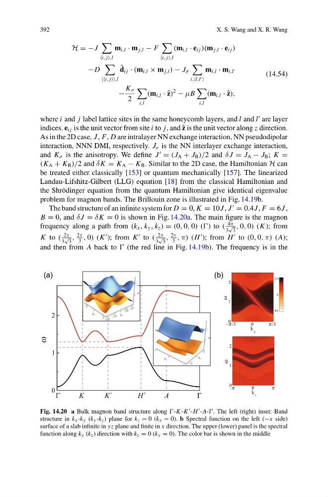
The band structure of an infinite system for D = 0, K = 10J , J
= 0.4J , F = 6J ,
B = 0, and δ J = δK = 0 is shown in Fig. 14.20a. The main figure is the magnon
frequency along a path from (k x , k y , k z ) = (0, 0, 0) () to (
4π
3
√
3
, 0, 0) (K ); from
K to (
2π
3
√
3
,
2π
3
, 0) (K
); from K
to (
2π
3
√
3
,
2π
3
, π) (H
); from H
to (0, 0, π) (A);
and then from A back to (the red line in Fig. 14.19b). The frequency is in the
K
K
H
A
2
1
0
0
k z
2
1
0
0
/3
/3
k y
4.0
0
4.9
(a)
(b)
Fig. 14.20 a Bulk magnon band structure along -K -H -A-. The left (right) inset: Band
structure in k x -k y (k y -k z ) plane for k z = 0 (k x = 0). b Spectral function on the left (−x side)
surface of a slab infinite in yz plane and finite in x direction. The upper (lower) panel is the spectral
function along k y (k z ) direction with k z = 0 (k y = 0). The color bar is shown in the middle
X. S. Wang and X. R. Wang
H = −J
j
m i,l · m j,l − F
j
(m i,l · e i j )(m j,l · e i j )
−D
j
ˆ
d i j · (m i,l × m j,l ) − J σ
i,
m i,l · m i,l
−
K σ
2
i,l
(m i,l · ˆ
z)
2
− μB
i,l
(m i,l · ˆ
z),
(14.54)
where i and j label lattice sites in the same honeycomb layers, and l and l
are layer
indices. e i j is the unit vector from site i to j, and ˆ
z is the unit vector along z direction.
As in the 2D case, J , F, D are intralayer NN exchange interaction, NN pseudodipolar
interaction, NNN DMI, respectively. J σ is the NN interlayer exchange interaction,
and K σ is the anisotropy. We define J
= (J A + J B )/2 and δ J = J A − J B ; K =
(K A + K B )/2 and δK = K A − K B . Similar to the 2D case, the Hamiltonian H can
be treated either classically [153] or quantum mechanically [157]. The linearized
Landau-Lifshitz-Gilbert (LLG) equation [18] from the classical Hamiltonian and
the Shrödinger equation from the quantum Hamiltonian give identical eigenvalue
problem for magnon bands. The Brillouin zone is illustrated in Fig. 14.19b.
The band structure of an infinite system for D = 0, K = 10J , J
= 0.4J , F = 6J ,
B = 0, and δ J = δK = 0 is shown in Fig. 14.20a. The main figure is the magnon
frequency along a path from (k x , k y , k z ) = (0, 0, 0) () to (
4π
3
√
3
, 0, 0) (K ); from
K to (
2π
3
√
3
,
2π
3
, 0) (K
); from K
to (
2π
3
√
3
,
2π
3
, π) (H
); from H
to (0, 0, π) (A);
and then from A back to (the red line in Fig. 14.19b). The frequency is in the
K
K
H
A
2
1
0
0
k z
2
1
0
0
/3
/3
k y
4.0
0
4.9
(a)
(b)
Fig. 14.20 a Bulk magnon band structure along -K -H -A-. The left (right) inset: Band
structure in k x -k y (k y -k z ) plane for k z = 0 (k x = 0). b Spectral function on the left (−x side)
surface of a slab infinite in yz plane and finite in x direction. The upper (lower) panel is the spectral
function along k y (k z ) direction with k z = 0 (k y = 0). The color bar is shown in the middle