

14 Topology in Magnetism
385
∂m i
∂t
= −m i ×
J
j
m j + F
j
(m j · e i j )e i j + K m iz e z + Be z
,
(14.45)
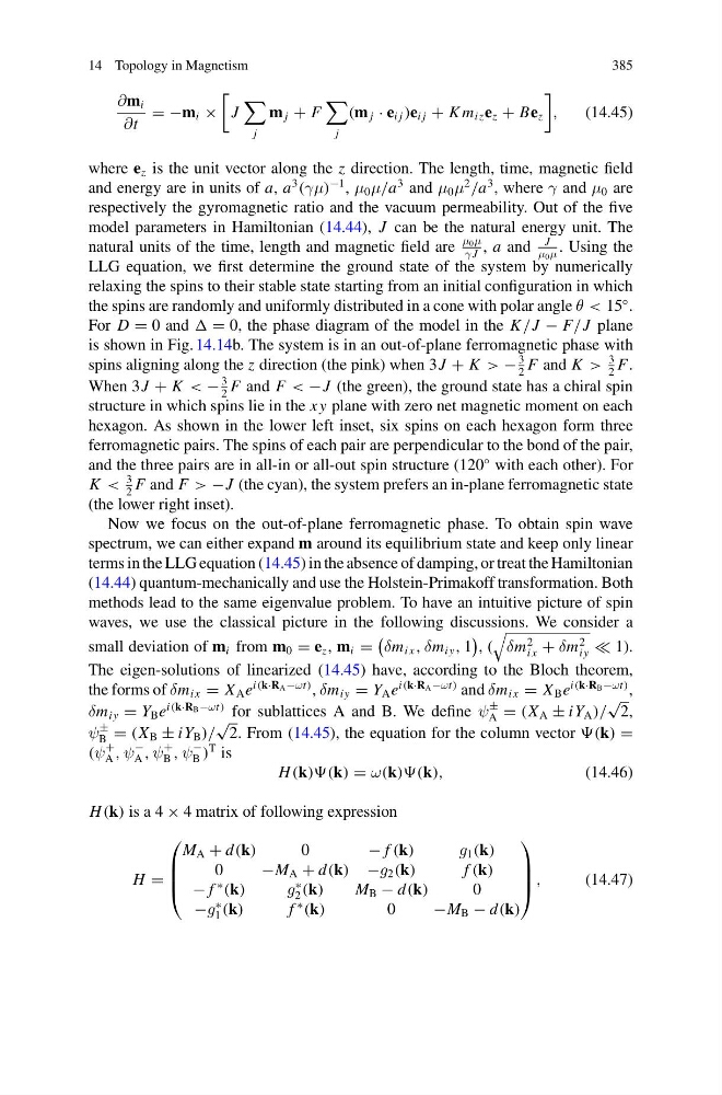
where e z is the unit vector along the z direction. The length, time, magnetic field
and energy are in units of a, a
3
(γμ)
−1 , μ 0 μ/a
3 and μ 0 μ
2
/a
3 , where γ and μ 0 are
respectively the gyromagnetic ratio and the vacuum permeability. Out of the five
model parameters in Hamiltonian (14.44), J can be the natural energy unit. The
natural units of the time, length and magnetic field are
μ 0 μ
γ J
, a and
J
μ 0 μ
. Using the
LLG equation, we first determine the ground state of the system by numerically
relaxing the spins to their stable state starting from an initial configuration in which
the spins are randomly and uniformly distributed in a cone with polar angle θ < 15
◦ .
For D = 0 and = 0, the phase diagram of the model in the K /J − F/J plane
is shown in Fig. 14.14b. The system is in an out-of-plane ferromagnetic phase with
spins aligning along the z direction (the pink) when 3J + K > −
3
2
F and K >
3
2
F.
When 3J + K < −
3
2
F and F < −J (the green), the ground state has a chiral spin
structure in which spins lie in the x y plane with zero net magnetic moment on each
hexagon. As shown in the lower left inset, six spins on each hexagon form three
ferromagnetic pairs. The spins of each pair are perpendicular to the bond of the pair,
and the three pairs are in all-in or all-out spin structure (120
◦ with each other). For
K <
3
2
F and F > −J (the cyan), the system prefers an in-plane ferromagnetic state
(the lower right inset).
Now we focus on the out-of-plane ferromagnetic phase. To obtain spin wave
spectrum, we can either expand m around its equilibrium state and keep only linear
terms in the LLG equation (14.45) in the absence of damping, or treat the Hamiltonian
(14.44) quantum-mechanically and use the Holstein-Primakoff transformation. Both
methods lead to the same eigenvalue problem. To have an intuitive picture of spin
waves, we use the classical picture in the following discussions. We consider a
small deviation of m i from m 0 = e z , m i =
δm i x , δm iy , 1
, (
δm
2
i x + δm
2
iy 1).
The eigen-solutions of linearized (14.45) have, according to the Bloch theorem,
the forms of δm i x = X A e
i(k·R A −ωt) , δm iy = Y A e
i(k·R A −ωt) and δm i x = X B e
i(k·R B −ωt) ,
δm iy = Y B e
i(k·R B −ωt) for sublattices A and B. We define ψ
±
A = (X A ± iY A )/
√
2,
ψ
±
B = (X B ± iY B )/
√
2. From (14.45), the equation for the column vector (k) =
(ψ
+
A , ψ
−
A , ψ
+
B , ψ
−
B )
T is
H (k))(k) = ω(k))(k),
(14.46)
H (k) is a 4 × 4 matrix of following expression
H =
⎛
⎜
⎜
⎝
M A + d(k)
0
− f (k)
g 1 (k)
0
−M A + d(k) −g 2 (k)
f (k)
− f
∗
(k)
g
∗
2 (k)
M B − d(k)
0
−g
∗
1 (k)
f
∗
(k)
0
−M B − d(k)
⎞
⎟
⎟
⎠ ,
(14.47)
385
∂m i
∂t
= −m i ×
J
j
m j + F
j
(m j · e i j )e i j + K m iz e z + Be z
,
(14.45)
where e z is the unit vector along the z direction. The length, time, magnetic field
and energy are in units of a, a
3
(γμ)
−1 , μ 0 μ/a
3 and μ 0 μ
2
/a
3 , where γ and μ 0 are
respectively the gyromagnetic ratio and the vacuum permeability. Out of the five
model parameters in Hamiltonian (14.44), J can be the natural energy unit. The
natural units of the time, length and magnetic field are
μ 0 μ
γ J
, a and
J
μ 0 μ
. Using the
LLG equation, we first determine the ground state of the system by numerically
relaxing the spins to their stable state starting from an initial configuration in which
the spins are randomly and uniformly distributed in a cone with polar angle θ < 15
◦ .
For D = 0 and = 0, the phase diagram of the model in the K /J − F/J plane
is shown in Fig. 14.14b. The system is in an out-of-plane ferromagnetic phase with
spins aligning along the z direction (the pink) when 3J + K > −
3
2
F and K >
3
2
F.
When 3J + K < −
3
2
F and F < −J (the green), the ground state has a chiral spin
structure in which spins lie in the x y plane with zero net magnetic moment on each
hexagon. As shown in the lower left inset, six spins on each hexagon form three
ferromagnetic pairs. The spins of each pair are perpendicular to the bond of the pair,
and the three pairs are in all-in or all-out spin structure (120
◦ with each other). For
K <
3
2
F and F > −J (the cyan), the system prefers an in-plane ferromagnetic state
(the lower right inset).
Now we focus on the out-of-plane ferromagnetic phase. To obtain spin wave
spectrum, we can either expand m around its equilibrium state and keep only linear
terms in the LLG equation (14.45) in the absence of damping, or treat the Hamiltonian
(14.44) quantum-mechanically and use the Holstein-Primakoff transformation. Both
methods lead to the same eigenvalue problem. To have an intuitive picture of spin
waves, we use the classical picture in the following discussions. We consider a
small deviation of m i from m 0 = e z , m i =
δm i x , δm iy , 1
, (
δm
2
i x + δm
2
iy 1).
The eigen-solutions of linearized (14.45) have, according to the Bloch theorem,
the forms of δm i x = X A e
i(k·R A −ωt) , δm iy = Y A e
i(k·R A −ωt) and δm i x = X B e
i(k·R B −ωt) ,
δm iy = Y B e
i(k·R B −ωt) for sublattices A and B. We define ψ
±
A = (X A ± iY A )/
√
2,
ψ
±
B = (X B ± iY B )/
√
2. From (14.45), the equation for the column vector (k) =
(ψ
+
A , ψ
−
A , ψ
+
B , ψ
−
B )
T is
H (k))(k) = ω(k))(k),
(14.46)
H (k) is a 4 × 4 matrix of following expression
H =
⎛
⎜
⎜
⎝
M A + d(k)
0
− f (k)
g 1 (k)
0
−M A + d(k) −g 2 (k)
f (k)
− f
∗
(k)
g
∗
2 (k)
M B − d(k)
0
−g
∗
1 (k)
f
∗
(k)
0
−M B − d(k)
⎞
⎟
⎟
⎠ ,
(14.47)