

13 Theoretical Generalization of the Optical Chirality to Arbitrary Optical Media
327
the sake of completeness, as well as for teaching purposes, we start from the basic
foundations. Hence, a proficient reader might skip the following part of the section.
In time domain, Poynting’s theorem can be directly obtained from the vector
identity ∇ · (A × B) = (∇ × A) · B − A · (∇ × B), along with the structural (or
curl-like) Maxwell’s equations ∇ × E = −∂ t B and ∇ × H = ∂ t D + J :
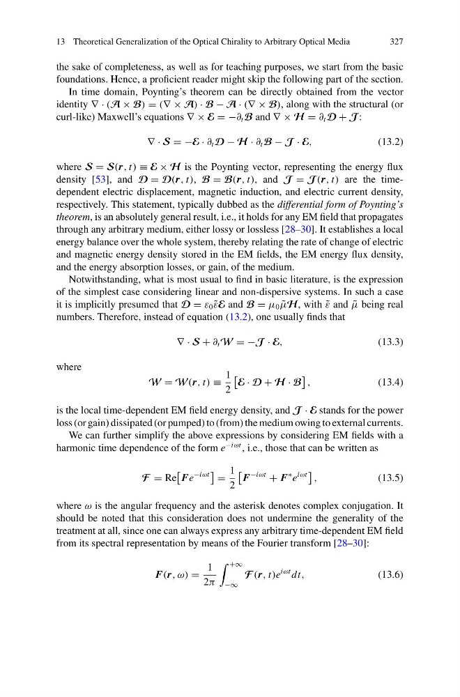
∇ · S = −E · ∂ t D − H · ∂ t B − J · E,
(13.2)
where S = S(r, t) ≡ E × H is the Poynting vector, representing the energy flux
density [53], and D = D(r, t), B = B(r, t), and J = J (r, t) are the timedependent electric displacement, magnetic induction, and electric current density,
respectively. This statement, typically dubbed as the differential form of Poynting’s
theorem, is an absolutely general result, i.e., it holds for any EM field that propagates
through any arbitrary medium, either lossy or lossless [28–30]. It establishes a local
energy balance over the whole system, thereby relating the rate of change of electric
and magnetic energy density stored in the EM fields, the EM energy flux density,
and the energy absorption losses, or gain, of the medium.
Notwithstanding, what is most usual to find in basic literature, is the expression
of the simplest case considering linear and non-dispersive systems. In such a case
it is implicitly presumed that D = ε 0 ˜
εE and B = μ 0 ˜
μH, with ˜
ε and ˜
μ being real
numbers. Therefore, instead of equation (13.2), one usually finds that
∇ · S + ∂ t W = −J · E,
(13.3)
where
W = W(r, t) ≡
1
2
E · D + H · B
,
(13.4)
is the local time-dependent EM field energy density, and J · E stands for the power
loss (or gain) dissipated (or pumped) to (from) the medium owing to external currents.
We can further simplify the above expressions by considering EM fields with a
harmonic time dependence of the form e
−iωt , i.e., those that can be written as
F = Re
Fe
−iωt
=
1
2
F
−iωt
+ F
∗ e
iωt
,
(13.5)
where ω is the angular frequency and the asterisk denotes complex conjugation. It
should be noted that this consideration does not undermine the generality of the
treatment at all, since one can always express any arbitrary time-dependent EM field
from its spectral representation by means of the Fourier transform [28–30]:
F(r, ω) =
1
2π
+∞
−∞
F (r, t)e
iωt dt,
(13.6)
327
the sake of completeness, as well as for teaching purposes, we start from the basic
foundations. Hence, a proficient reader might skip the following part of the section.
In time domain, Poynting’s theorem can be directly obtained from the vector
identity ∇ · (A × B) = (∇ × A) · B − A · (∇ × B), along with the structural (or
curl-like) Maxwell’s equations ∇ × E = −∂ t B and ∇ × H = ∂ t D + J :
∇ · S = −E · ∂ t D − H · ∂ t B − J · E,
(13.2)
where S = S(r, t) ≡ E × H is the Poynting vector, representing the energy flux
density [53], and D = D(r, t), B = B(r, t), and J = J (r, t) are the timedependent electric displacement, magnetic induction, and electric current density,
respectively. This statement, typically dubbed as the differential form of Poynting’s
theorem, is an absolutely general result, i.e., it holds for any EM field that propagates
through any arbitrary medium, either lossy or lossless [28–30]. It establishes a local
energy balance over the whole system, thereby relating the rate of change of electric
and magnetic energy density stored in the EM fields, the EM energy flux density,
and the energy absorption losses, or gain, of the medium.
Notwithstanding, what is most usual to find in basic literature, is the expression
of the simplest case considering linear and non-dispersive systems. In such a case
it is implicitly presumed that D = ε 0 ˜
εE and B = μ 0 ˜
μH, with ˜
ε and ˜
μ being real
numbers. Therefore, instead of equation (13.2), one usually finds that
∇ · S + ∂ t W = −J · E,
(13.3)
where
W = W(r, t) ≡
1
2
E · D + H · B
,
(13.4)
is the local time-dependent EM field energy density, and J · E stands for the power
loss (or gain) dissipated (or pumped) to (from) the medium owing to external currents.
We can further simplify the above expressions by considering EM fields with a
harmonic time dependence of the form e
−iωt , i.e., those that can be written as
F = Re
Fe
−iωt
=
1
2
F
−iωt
+ F
∗ e
iωt
,
(13.5)
where ω is the angular frequency and the asterisk denotes complex conjugation. It
should be noted that this consideration does not undermine the generality of the
treatment at all, since one can always express any arbitrary time-dependent EM field
from its spectral representation by means of the Fourier transform [28–30]:
F(r, ω) =
1
2π
+∞
−∞
F (r, t)e
iωt dt,
(13.6)