

9 Symmetry Approach to Chiral Optomagnonics in Antiferromagnetic Insulators
235
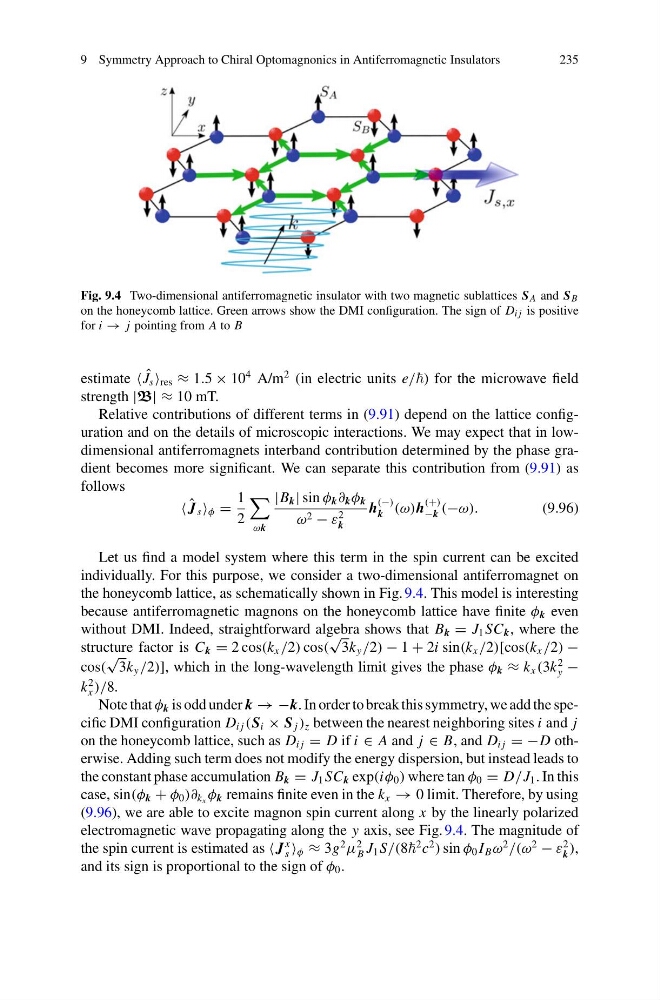
Fig. 9.4 Two-dimensional antiferromagnetic insulator with two magnetic sublattices S A and S B
on the honeycomb lattice. Green arrows show the DMI configuration. The sign of D i j is positive
for i → j pointing from A to B
estimate ˆ
J s res ≈ 1.5 × 10
4 A/m
2 (in electric units e/) for the microwave field
strength |B| ≈ 10 mT.
Relative contributions of different terms in (9.91) depend on the lattice configuration and on the details of microscopic interactions. We may expect that in lowdimensional antiferromagnets interband contribution determined by the phase gradient becomes more significant. We can separate this contribution from (9.91) as
follows
ˆ
J s φ =
1
2
ωk
|B k | sin φ k ∂ k φ k
ω 2 − ε
2
k
h
(−)
k (ω)h
(+)
−k (−ω).
(9.96)
Let us find a model system where this term in the spin current can be excited
individually. For this purpose, we consider a two-dimensional antiferromagnet on
the honeycomb lattice, as schematically shown in Fig. 9.4. This model is interesting
because antiferromagnetic magnons on the honeycomb lattice have finite φ k even
without DMI. Indeed, straightforward algebra shows that B k = J 1 SC k , where the
structure factor is C k = 2 cos(k x /2) cos(
√
3k y /2) − 1 + 2i sin(k x /2)[cos(k x /2) −
cos(
√
3k y /2)], which in the long-wavelength limit gives the phase φ k ≈ k x (3k
2
y −
k
2
x )/8.
Note that φ k is odd under k → −k. In order to break this symmetry, we add the specific DMI configuration D i j (S i × S j ) z between the nearest neighboring sites i and j
on the honeycomb lattice, such as D i j = D if i ∈ A and j ∈ B, and D i j = −D otherwise. Adding such term does not modify the energy dispersion, but instead leads to
the constant phase accumulation B k = J 1 SC k exp(iφ 0 ) where tan φ 0 = D/J 1 . In this
case, sin(φ k + φ 0 )∂ k x φ k remains finite even in the k x → 0 limit. Therefore, by using
(9.96), we are able to excite magnon spin current along x by the linearly polarized
electromagnetic wave propagating along the y axis, see Fig. 9.4. The magnitude of
the spin current is estimated as J
x
s φ ≈ 3g
2
μ
2
B J 1 S/(8
2 c
2
) sin φ 0 I B ω
2
/(ω
2
− ε
2
k ),
and its sign is proportional to the sign of φ 0 .
235
Fig. 9.4 Two-dimensional antiferromagnetic insulator with two magnetic sublattices S A and S B
on the honeycomb lattice. Green arrows show the DMI configuration. The sign of D i j is positive
for i → j pointing from A to B
estimate ˆ
J s res ≈ 1.5 × 10
4 A/m
2 (in electric units e/) for the microwave field
strength |B| ≈ 10 mT.
Relative contributions of different terms in (9.91) depend on the lattice configuration and on the details of microscopic interactions. We may expect that in lowdimensional antiferromagnets interband contribution determined by the phase gradient becomes more significant. We can separate this contribution from (9.91) as
follows
ˆ
J s φ =
1
2
ωk
|B k | sin φ k ∂ k φ k
ω 2 − ε
2
k
h
(−)
k (ω)h
(+)
−k (−ω).
(9.96)
Let us find a model system where this term in the spin current can be excited
individually. For this purpose, we consider a two-dimensional antiferromagnet on
the honeycomb lattice, as schematically shown in Fig. 9.4. This model is interesting
because antiferromagnetic magnons on the honeycomb lattice have finite φ k even
without DMI. Indeed, straightforward algebra shows that B k = J 1 SC k , where the
structure factor is C k = 2 cos(k x /2) cos(
√
3k y /2) − 1 + 2i sin(k x /2)[cos(k x /2) −
cos(
√
3k y /2)], which in the long-wavelength limit gives the phase φ k ≈ k x (3k
2
y −
k
2
x )/8.
Note that φ k is odd under k → −k. In order to break this symmetry, we add the specific DMI configuration D i j (S i × S j ) z between the nearest neighboring sites i and j
on the honeycomb lattice, such as D i j = D if i ∈ A and j ∈ B, and D i j = −D otherwise. Adding such term does not modify the energy dispersion, but instead leads to
the constant phase accumulation B k = J 1 SC k exp(iφ 0 ) where tan φ 0 = D/J 1 . In this
case, sin(φ k + φ 0 )∂ k x φ k remains finite even in the k x → 0 limit. Therefore, by using
(9.96), we are able to excite magnon spin current along x by the linearly polarized
electromagnetic wave propagating along the y axis, see Fig. 9.4. The magnitude of
the spin current is estimated as J
x
s φ ≈ 3g
2
μ
2
B J 1 S/(8
2 c
2
) sin φ 0 I B ω
2
/(ω
2
− ε
2
k ),
and its sign is proportional to the sign of φ 0 .