

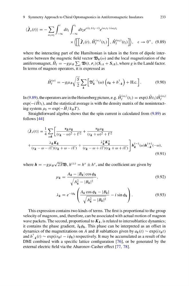
9 Symmetry Approach to Chiral Optomagnonics in Antiferromagnetic Insulators
233
ˆ
J s (t) = −
ω 1 ω 2
t
−∞
dt 1
t 1
−∞
dt 2 e
(t 1 +t 2 −t) e
iω 1 t 1 +iω 2 t 2
×
ˆ
J s (t), ˆ
H
(ω 1 )
I
(t 1 )
, ˆ
H
(ω 2 )
I
(t 2 )
, , → 0
+
, (9.89)
where the interacting part of the Hamiltonian is taken in the form of dipole interaction between the magnetic field vector B k (ω) and the local magnetization of the
antiferromagnet, ˆ
H I = −gμ B
i B(t, r i )(S i A + S i B ), where g is the Landé factor.
In terms of magnon operators, it is expressed as
ˆ
H
(ω)
I
= −gμ B
S
2
k
B
(−)
k (ω)
a k + b
†
−k
+ H.c.
.
(9.90)
In (9.89), the operators are in the Heisenberg picture, e.g. ˆ
H
(ω 1 )
I
(t 1 ) = exp(i ˆ
Ht 1 ) ˆ
H
(ω 1 )
I
exp(−i ˆ
Ht 1 ), and the statistical average is with the density matrix of the noninteracting system ρ 0 = exp(− ˆ
H /k B T ).
Straightforward algebra shows that the spin current is calculated from (9.89) as
follows [44]
ˆ
J s (t) =
1
4
ωk
v k μ k
(ε k − ω) 2 + 2 +
v k μ k
(ε k + ω) 2 + 2
+
λ k K k
(ε k − ω − i)(ε k + ω − i)
+
λ ∗
k K ∗
k
(ε k − ω + i)(ε k + ω + i)
h
(−)
k (ω)h
(+)
−k (−ω),
(9.91)
where h = −gμ B
√
2SB, h
(±)
= h
x
± h
y , and the coefficient are given by
μ k =
A k − |B k | cos φ k
A
2
k − |B k | 2
,
(9.92)
λ k = e
−iφ k
⎛
⎝ A k cos φ k − |B k |
A
2
k − |B k | 2
− i sin φ k
⎞
⎠ .
(9.93)
This expression contains two kinds of terms. The first is proportional to the group
velocity of magnons, and, therefore, can be associated with actual motion of magnon
wave packets. The second, proportional to K k , is related to intersublattice dynamics;
it contains the phase gradient, ∂ k φ k . This phase can be interpreted as an offset in
dynamics of the magnetizations on A and B sublattices given by a k (t) ∼ exp(iε k t)
and b
†
−k (t) ∼ exp(iε k t − iφ k ) respectively. It may be accumulated as a result of the
DMI combined with a specific lattice configuration [76], or be generated by the
external electric field via the Aharonov-Casher effect [77, 78].
233
ˆ
J s (t) = −
ω 1 ω 2
t
−∞
dt 1
t 1
−∞
dt 2 e
(t 1 +t 2 −t) e
iω 1 t 1 +iω 2 t 2
×
ˆ
J s (t), ˆ
H
(ω 1 )
I
(t 1 )
, ˆ
H
(ω 2 )
I
(t 2 )
, , → 0
+
, (9.89)
where the interacting part of the Hamiltonian is taken in the form of dipole interaction between the magnetic field vector B k (ω) and the local magnetization of the
antiferromagnet, ˆ
H I = −gμ B
i B(t, r i )(S i A + S i B ), where g is the Landé factor.
In terms of magnon operators, it is expressed as
ˆ
H
(ω)
I
= −gμ B
S
2
k
B
(−)
k (ω)
a k + b
†
−k
+ H.c.
.
(9.90)
In (9.89), the operators are in the Heisenberg picture, e.g. ˆ
H
(ω 1 )
I
(t 1 ) = exp(i ˆ
Ht 1 ) ˆ
H
(ω 1 )
I
exp(−i ˆ
Ht 1 ), and the statistical average is with the density matrix of the noninteracting system ρ 0 = exp(− ˆ
H /k B T ).
Straightforward algebra shows that the spin current is calculated from (9.89) as
follows [44]
ˆ
J s (t) =
1
4
ωk
v k μ k
(ε k − ω) 2 + 2 +
v k μ k
(ε k + ω) 2 + 2
+
λ k K k
(ε k − ω − i)(ε k + ω − i)
+
λ ∗
k K ∗
k
(ε k − ω + i)(ε k + ω + i)
h
(−)
k (ω)h
(+)
−k (−ω),
(9.91)
where h = −gμ B
√
2SB, h
(±)
= h
x
± h
y , and the coefficient are given by
μ k =
A k − |B k | cos φ k
A
2
k − |B k | 2
,
(9.92)
λ k = e
−iφ k
⎛
⎝ A k cos φ k − |B k |
A
2
k − |B k | 2
− i sin φ k
⎞
⎠ .
(9.93)
This expression contains two kinds of terms. The first is proportional to the group
velocity of magnons, and, therefore, can be associated with actual motion of magnon
wave packets. The second, proportional to K k , is related to intersublattice dynamics;
it contains the phase gradient, ∂ k φ k . This phase can be interpreted as an offset in
dynamics of the magnetizations on A and B sublattices given by a k (t) ∼ exp(iε k t)
and b
†
−k (t) ∼ exp(iε k t − iφ k ) respectively. It may be accumulated as a result of the
DMI combined with a specific lattice configuration [76], or be generated by the
external electric field via the Aharonov-Casher effect [77, 78].