

212
I. Proskurin and R. L. Stamps
E(t, r) =
1
(2π) 3/2
d
3 pe
i p·r E(t, p),
(9.10)
B(t, r) =
1
(2π) 3/2
d
3 pe
i p·r B(t, p).
(9.11)
The matrix on the right-hand side of equation (9.9) has the following structure
H( p) =
0
i( ˆ
S · p)
−i( ˆ
S · p)
0
,
(9.12)
which can be considered as a direct product of the Pauli matrix σ 2 , which interchanges
E and B, and the “helicity” operator ( ˆ
S · p), where the matrices ˆ
S α (α = x, y, z)
form a representation of the three-dimensional rotation group, ( ˆ
S α ) βγ = i αβγ , with
αβγ being the Levi-Civita symbol.
The second pair of the Maxwell’s equations (9.5) in this formalism impose an
additional constraint on the components of φ(t, p) [18]
( ˆ
S · p)
2
φ(t, p) = p
2
φ(t, p),
(9.13)
which acknowledges transversality of the electromagnetic field in vacuum.
9.2.1.1 Invariance Algebra of the Maxwell’s Equations
Now, we can find the symmetry operations that transform a solution φ(t, p) of (9.9)
into another solution ˜
φ(t, p) = Q( p)φ(t, p). We look for these transformations in
the form of the six-dimensional matrices Q( p), which may depend on the momentum
p. Formal resemblance of our representation with the quantum mechanics implies
that these matrices should commute with H( p).
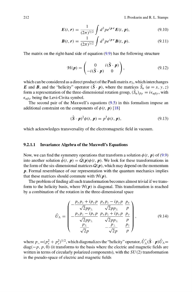
The problem of finding all such transformation becomes almost trivial if we transform to the helicity basis, where H( p) is diagonal. This transformation is reached
by a combination of the rotation in the three-dimensional space
ˆ
U =
⎛
⎜
⎜
⎜
⎜
⎜
⎜
⎝
−
p x p z + i p y p
√
2 pp ⊥
p x p z − i p y p
√
2 pp ⊥
p x
p
−
p y p z − i p x p
√
2 pp ⊥
p y p z + i p x p
√
2 pp ⊥
p y
p
p ⊥
√
2 p
−
p ⊥
√
2 p
p z
p
⎞
⎟
⎟
⎟
⎟
⎟
⎟
⎠
,
(9.14)
where p ⊥ =( p
2
x + p
2
y )
1/2 , which diagonalizes the “helicity” operator, ˆ
U
†
( ˆ
S · p) ˆ
U =
diag(− p, p, 0) (it transforms to the basis where the electric and magnetic fields are
written in terms of circularly polarized components), with the SU (2) transformation
in the pseudo-space of electric and magnetic fields
I. Proskurin and R. L. Stamps
E(t, r) =
1
(2π) 3/2
d
3 pe
i p·r E(t, p),
(9.10)
B(t, r) =
1
(2π) 3/2
d
3 pe
i p·r B(t, p).
(9.11)
The matrix on the right-hand side of equation (9.9) has the following structure
H( p) =
0
i( ˆ
S · p)
−i( ˆ
S · p)
0
,
(9.12)
which can be considered as a direct product of the Pauli matrix σ 2 , which interchanges
E and B, and the “helicity” operator ( ˆ
S · p), where the matrices ˆ
S α (α = x, y, z)
form a representation of the three-dimensional rotation group, ( ˆ
S α ) βγ = i αβγ , with
αβγ being the Levi-Civita symbol.
The second pair of the Maxwell’s equations (9.5) in this formalism impose an
additional constraint on the components of φ(t, p) [18]
( ˆ
S · p)
2
φ(t, p) = p
2
φ(t, p),
(9.13)
which acknowledges transversality of the electromagnetic field in vacuum.
9.2.1.1 Invariance Algebra of the Maxwell’s Equations
Now, we can find the symmetry operations that transform a solution φ(t, p) of (9.9)
into another solution ˜
φ(t, p) = Q( p)φ(t, p). We look for these transformations in
the form of the six-dimensional matrices Q( p), which may depend on the momentum
p. Formal resemblance of our representation with the quantum mechanics implies
that these matrices should commute with H( p).
The problem of finding all such transformation becomes almost trivial if we transform to the helicity basis, where H( p) is diagonal. This transformation is reached
by a combination of the rotation in the three-dimensional space
ˆ
U =
⎛
⎜
⎜
⎜
⎜
⎜
⎜
⎝
−
p x p z + i p y p
√
2 pp ⊥
p x p z − i p y p
√
2 pp ⊥
p x
p
−
p y p z − i p x p
√
2 pp ⊥
p y p z + i p x p
√
2 pp ⊥
p y
p
p ⊥
√
2 p
−
p ⊥
√
2 p
p z
p
⎞
⎟
⎟
⎟
⎟
⎟
⎟
⎠
,
(9.14)
where p ⊥ =( p
2
x + p
2
y )
1/2 , which diagonalizes the “helicity” operator, ˆ
U
†
( ˆ
S · p) ˆ
U =
diag(− p, p, 0) (it transforms to the basis where the electric and magnetic fields are
written in terms of circularly polarized components), with the SU (2) transformation
in the pseudo-space of electric and magnetic fields