

6 Magnetoelectricity of Chiral Micromagnetic Structures
143
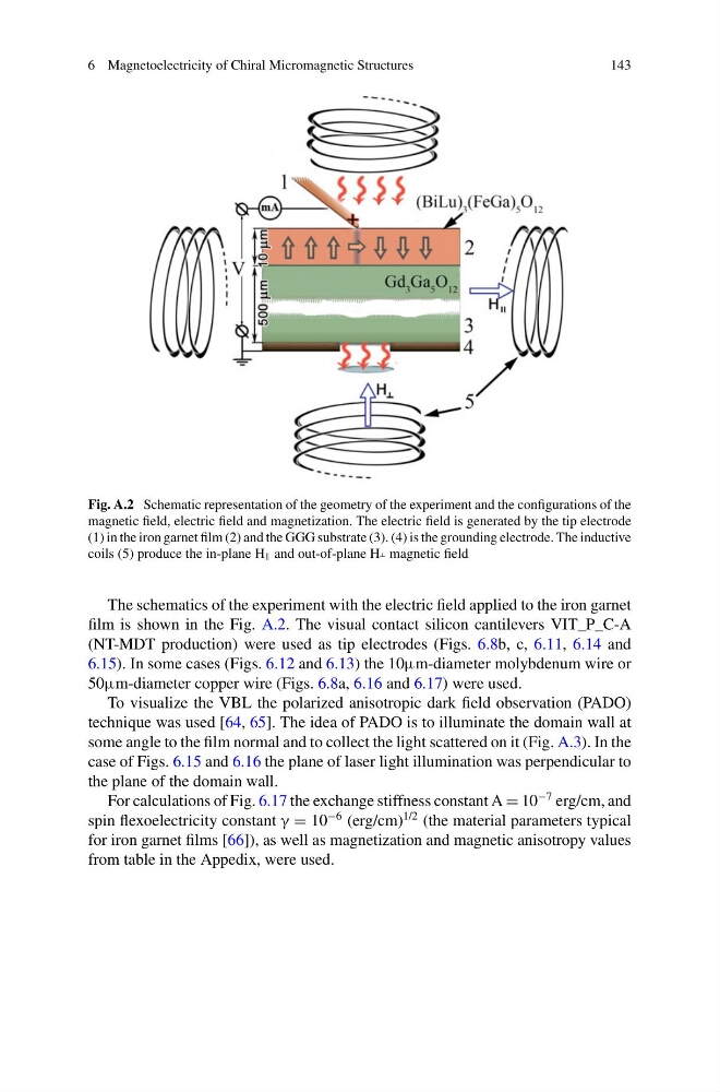
Fig. A.2 Schematic representation of the geometry of the experiment and the configurations of the
magnetic field, electric field and magnetization. The electric field is generated by the tip electrode
(1) in the iron garnet film (2) and the GGG substrate (3). (4) is the grounding electrode. The inductive
coils (5) produce the in-plane H and out-of-plane H magnetic field
The schematics of the experiment with the electric field applied to the iron garnet
film is shown in the Fig. A.2. The visual contact silicon cantilevers VIT_P_C-A
(NT-MDT production) were used as tip electrodes (Figs. 6.8b, c, 6.11, 6.14 and
6.15). In some cases (Figs. 6.12 and 6.13) the 10μm-diameter molybdenum wire or
50μm-diameter copper wire (Figs. 6.8a, 6.16 and 6.17) were used.
To visualize the VBL the polarized anisotropic dark field observation (PADO)
technique was used [64, 65]. The idea of PADO is to illuminate the domain wall at
some angle to the film normal and to collect the light scattered on it (Fig. A.3). In the
case of Figs. 6.15 and 6.16 the plane of laser light illumination was perpendicular to
the plane of the domain wall.
For calculations of Fig. 6.17 the exchange stiffness constant A = 10
−7 erg/cm, and
spin flexoelectricity constant γ = 10
−6 (erg/cm)
1/2 (the material parameters typical
for iron garnet films [66]), as well as magnetization and magnetic anisotropy values
from table in the Appedix, were used.
143
Fig. A.2 Schematic representation of the geometry of the experiment and the configurations of the
magnetic field, electric field and magnetization. The electric field is generated by the tip electrode
(1) in the iron garnet film (2) and the GGG substrate (3). (4) is the grounding electrode. The inductive
coils (5) produce the in-plane H and out-of-plane H magnetic field
The schematics of the experiment with the electric field applied to the iron garnet
film is shown in the Fig. A.2. The visual contact silicon cantilevers VIT_P_C-A
(NT-MDT production) were used as tip electrodes (Figs. 6.8b, c, 6.11, 6.14 and
6.15). In some cases (Figs. 6.12 and 6.13) the 10μm-diameter molybdenum wire or
50μm-diameter copper wire (Figs. 6.8a, 6.16 and 6.17) were used.
To visualize the VBL the polarized anisotropic dark field observation (PADO)
technique was used [64, 65]. The idea of PADO is to illuminate the domain wall at
some angle to the film normal and to collect the light scattered on it (Fig. A.3). In the
case of Figs. 6.15 and 6.16 the plane of laser light illumination was perpendicular to
the plane of the domain wall.
For calculations of Fig. 6.17 the exchange stiffness constant A = 10
−7 erg/cm, and
spin flexoelectricity constant γ = 10
−6 (erg/cm)
1/2 (the material parameters typical
for iron garnet films [66]), as well as magnetization and magnetic anisotropy values
from table in the Appedix, were used.