

344
R. dell’Erba
line on its left; this because, in this case, the leaders have in their neighbors, some
points of the frame that always are close to them. We can avoid this convexity effect
using a different frame or mirroring the followers to obtain an infinite sample. This
is also evident in Fig. 18.9 where contiguous configurations are compared using the
PE2 formula.
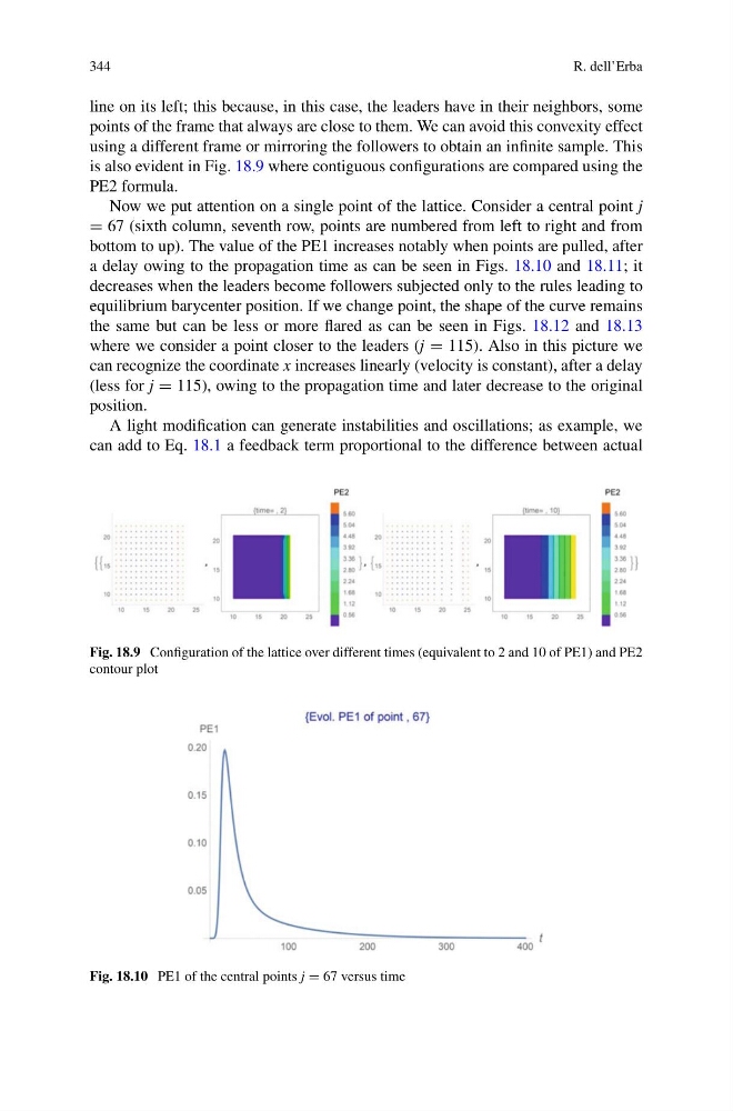
Now we put attention on a single point of the lattice. Consider a central point j
= 67 (sixth column, seventh row, points are numbered from left to right and from
bottom to up). The value of the PE1 increases notably when points are pulled, after
a delay owing to the propagation time as can be seen in Figs. 18.10 and 18.11; it
decreases when the leaders become followers subjected only to the rules leading to
equilibrium barycenter position. If we change point, the shape of the curve remains
the same but can be less or more flared as can be seen in Figs. 18.12 and 18.13
where we consider a point closer to the leaders (j = 115). Also in this picture we
can recognize the coordinate x increases linearly (velocity is constant), after a delay
(less for j = 115), owing to the propagation time and later decrease to the original
position.
A light modification can generate instabilities and oscillations; as example, we
can add to Eq. 18.1 a feedback term proportional to the difference between actual
Fig. 18.9 Configuration of the lattice over different times (equivalent to 2 and 10 of PE1) and PE2
contour plot
Fig. 18.10 PE1 of the central points j = 67 versus time
R. dell’Erba
line on its left; this because, in this case, the leaders have in their neighbors, some
points of the frame that always are close to them. We can avoid this convexity effect
using a different frame or mirroring the followers to obtain an infinite sample. This
is also evident in Fig. 18.9 where contiguous configurations are compared using the
PE2 formula.
Now we put attention on a single point of the lattice. Consider a central point j
= 67 (sixth column, seventh row, points are numbered from left to right and from
bottom to up). The value of the PE1 increases notably when points are pulled, after
a delay owing to the propagation time as can be seen in Figs. 18.10 and 18.11; it
decreases when the leaders become followers subjected only to the rules leading to
equilibrium barycenter position. If we change point, the shape of the curve remains
the same but can be less or more flared as can be seen in Figs. 18.12 and 18.13
where we consider a point closer to the leaders (j = 115). Also in this picture we
can recognize the coordinate x increases linearly (velocity is constant), after a delay
(less for j = 115), owing to the propagation time and later decrease to the original
position.
A light modification can generate instabilities and oscillations; as example, we
can add to Eq. 18.1 a feedback term proportional to the difference between actual
Fig. 18.9 Configuration of the lattice over different times (equivalent to 2 and 10 of PE1) and PE2
contour plot
Fig. 18.10 PE1 of the central points j = 67 versus time