

17 Microplane Modeling for Inelastic Responses …
307
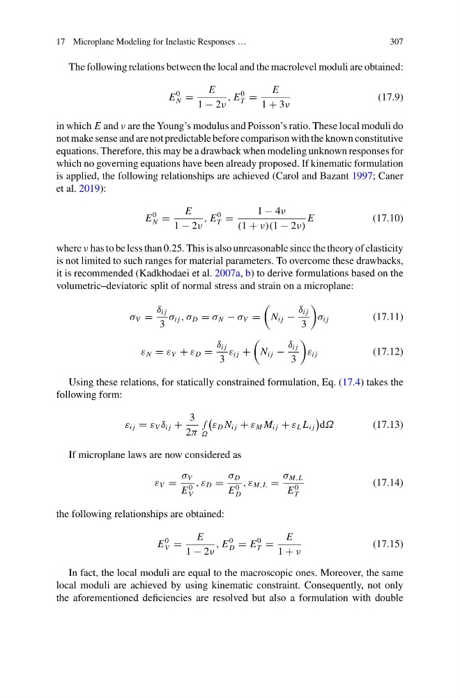
The following relations between the local and the macrolevel moduli are obtained:
E
0
N =
E
1 − 2ν
, E
0
T =
E
1 + 3ν
(17.9)
in which E and ν are the Young’s modulus and Poisson’s ratio. These local moduli do
not make sense and are not predictable before comparison with the known constitutive
equations. Therefore, this may be a drawback when modeling unknown responses for
which no governing equations have been already proposed. If kinematic formulation
is applied, the following relationships are achieved (Carol and Bazant 1997; Caner
et al. 2019):
E
0
N =
E
1 − 2ν
, E
0
T =
1 − 4ν
(1 + ν)(1 − 2ν)
E
(17.10)
where ν has to be less than 0.25. This is also unreasonable since the theory of elasticity
is not limited to such ranges for material parameters. To overcome these drawbacks,
it is recommended (Kadkhodaei et al. 2007a, b) to derive formulations based on the
volumetric–deviatoric split of normal stress and strain on a microplane:
σ V =
δ i j
3
σ i j , σ D = σ N − σ V =
N i j −
δ i j
3
σ i j
(17.11)
ε N = ε V + ε D =
δ i j
3
ε i j +
N i j −
δ i j
3
ε i j
(17.12)
Using these relations, for statically constrained formulation, Eq. (17.4) takes the
following form:
ε i j = ε V δ i j +
3
2π
∫
Ω
ε D N i j + ε M M i j + ε L L i j
dΩ
(17.13)
If microplane laws are now considered as
ε V =
σ V
E
0
V
, ε D =
σ D
E
0
D
, ε M,L =
σ M,L
E
0
T
(17.14)
the following relationships are obtained:
E
0
V =
E
1 − 2ν
, E
0
D = E
0
T =
E
1 + ν
(17.15)
In fact, the local moduli are equal to the macroscopic ones. Moreover, the same
local moduli are achieved by using kinematic constraint. Consequently, not only
the aforementioned deficiencies are resolved but also a formulation with double
307
The following relations between the local and the macrolevel moduli are obtained:
E
0
N =
E
1 − 2ν
, E
0
T =
E
1 + 3ν
(17.9)
in which E and ν are the Young’s modulus and Poisson’s ratio. These local moduli do
not make sense and are not predictable before comparison with the known constitutive
equations. Therefore, this may be a drawback when modeling unknown responses for
which no governing equations have been already proposed. If kinematic formulation
is applied, the following relationships are achieved (Carol and Bazant 1997; Caner
et al. 2019):
E
0
N =
E
1 − 2ν
, E
0
T =
1 − 4ν
(1 + ν)(1 − 2ν)
E
(17.10)
where ν has to be less than 0.25. This is also unreasonable since the theory of elasticity
is not limited to such ranges for material parameters. To overcome these drawbacks,
it is recommended (Kadkhodaei et al. 2007a, b) to derive formulations based on the
volumetric–deviatoric split of normal stress and strain on a microplane:
σ V =
δ i j
3
σ i j , σ D = σ N − σ V =
N i j −
δ i j
3
σ i j
(17.11)
ε N = ε V + ε D =
δ i j
3
ε i j +
N i j −
δ i j
3
ε i j
(17.12)
Using these relations, for statically constrained formulation, Eq. (17.4) takes the
following form:
ε i j = ε V δ i j +
3
2π
∫
Ω
ε D N i j + ε M M i j + ε L L i j
dΩ
(17.13)
If microplane laws are now considered as
ε V =
σ V
E
0
V
, ε D =
σ D
E
0
D
, ε M,L =
σ M,L
E
0
T
(17.14)
the following relationships are obtained:
E
0
V =
E
1 − 2ν
, E
0
D = E
0
T =
E
1 + ν
(17.15)
In fact, the local moduli are equal to the macroscopic ones. Moreover, the same
local moduli are achieved by using kinematic constraint. Consequently, not only
the aforementioned deficiencies are resolved but also a formulation with double